Introduction
In this section we cover the open source SASPy module from SAS Institute. It exposes Python APIs to Base SAS and allows a Python session to do the following:
• Start and connect to a local or remote SAS session
• Enable bi-directional transfer of values between SAS variables and Python objects
• Enables bi-directional exchange of data between pandas DataFrames and SAS datasets
• Enable bi-directional exchange of SAS Macro variables and Python objects
• Integrate SAS and Python program logic within a single execution context interactively or batch (scripted) mode
To get started take the following steps:
1. Install the saspy module
2. Set-up the sascfg_personal.py configuration file
3. Make the SAS-supplied Java .jar files available to SASPy
These instructions are for Windows.
Install SASPy
Issue the following command in a Windows terminal session:
python -m pip install saspy
The installation process downloads SASPy and its dependent packages.
Collecting saspy
  Downloading https://files.pythonhosted.org/packages/bb/07/3fd96b969959ef0e701e5764f6a239e7bea543b37d2d7a81acb23ed6a0c5/saspy-2.2.9.tar.gz (97kB)
    100% |████████████████████████████████| 102kB 769kB/s
Successfully built saspy
distributed 1.21.8 requires msgpack, which is not installed.
Installing collected packages: saspy
Successfully installed saspy-2.2.9
Modify sascfg_personal.py Configuration File
Here we configure an IOM (integrated object model) connection method so the Python session running on Windows connects to a SAS session running on the same Windows machine. If you have a different set-up, for example, Python on Windows connecting to a SAS session on Linux, use the STDIO access method.
Detailed instructions are here. In this case, we are configuring a local connection. Details for this configuration are located here. Even better is the autocfg.py script the clever guys at SAS published to help get you going quickly.
Locate the SASPy.SAScfg Configuration File.
import saspy
saspy
<module 'saspy.sascfg' from 'C:\\Users\\randy\\Anaconda3\\lib\\site-packages\\saspy\\sascfg.py'>
Copy the sascfg.py configuration file to sascfg_personal.py. This ensures that any configuration changes will not be overwritten when subsequent versions of SASPy are installed later.
In this example we copied:
C:/Users/randy/Anaconda3/lib/site-packages/saspy/sascfg.py
to
C:/Users/randy/Anaconda3/lib/site-packages/saspy /personal_sascfg.py
From the original sascfg.py configuration file:
SAS_config_names=['default']
we changed in the sascfg_personal.py configuration file to:
SAS_config_names=['winlocal']
Make SAS-supplied .jar Files Available
These .jar files are needed by SASPy and must be defined by the classpath variable in the sascfg_personal.py configuration file:
sas.svc.connection.jar
log4j.jar
sas.security.sspi.jar
sas.core.jar
These four .jar files are part of the existing SAS deployment. Depending on where SAS is installed on Windows the path will be something like:
C:\Program Files\SASHome\SASDeploymentManager\9.4\products\deploywiz__94498__prt__xx__sp0__1\deploywiz\<required_jar_file_names.jar>
A fifth .jar file is distributed with the SASPy repo; saspyiom.jar must be defined as part of the classpath variable in the sascfg_personal.py configuration file as well. In our case this jar file was located at:
C:/Users/randy/Anaconda3/Lib/site-packages/saspy/java
Once you have the location of these .jar files, modify the sascfg_personal.py file CLASSPATH variable in the SAScfg_personal.py file similar to:
# build out a local classpath variable to use below for Windows clients

cpW  =  "C:\\Program Files\\SASHome\\SASDeploymentManager\\9.4\\products\\deploywiz__94498__prt__xx__sp0__1\\deploywiz\\sas.svc.connection.jar"

cpW += ";C:\\Program Files\\SASHome\\SASDeploymentManager\\9.4\\products\\deploywiz__94498__prt__xx__sp0__1\\deploywiz\\log4j.jar"

cpW += ";C:\\Program Files\\SASHome\\SASDeploymentManager\\9.4\\products\\deploywiz__94498__prt__xx__sp0__1\\deploywiz\\sas.security.sspi.jar"

cpW += ";C:\\Program Files\\SASHome\\SASDeploymentManager\\9.4\\products\\deploywiz__94498__prt__xx__sp0__1\\deploywiz\\sas.core.jar"

cpW += ";C:\\Users\\randy\\Anaconda3\\Lib\\site-packages\\saspy\\java\\saspyiom.jar"
Be sure to modify the paths sepcific to your environment.
SASPy has a dependency on Java 7 met by relying on the SAS Private JRE distributed and installed with SAS.
To have SASPy recognize this JRE update the dictionary values for the winlocal object definition in the sascfg_personal.py configuration file similar to:
winlocal = {'java'  : 'C:\\Program Files\\SASHome\\SASPrivateJavaRuntimeEnvironment\\9.4\\jre\\bin\\java',
            'encoding'  : 'windows-1252',
            'classpath' : cpW
            }
Notice the path filename uses double back-slashes to ‘escape’ the backslash needed by the Windows path names.
There is one final requirement. The `sspiauth.dll file–also included in the SAS installation–must be a part of the system PATH environment variable, java.library.path, or in the home directory of the Java client. Search for this file in your SAS deployment, though it is likely in SASHome\SASFoundation\9.4\core\sasext.
Examples
Call SASPy and connect to a SAS session to creathe the sas object and calling the saspy.SASsession object.
import pandas as pd
import saspy
import numpy as np
from IPython.display import HTML

sas = saspy.SASsession(results='HTML')
Using SAS Config named: winlocal
SAS Connection established. Subprocess id is 15752
Most of the arguments to the SASsession object are set in the sascfg_personal.py configuration file discussed above.
The results= argument uses three values to indicate how tabular output returned from the SASsession object, that is, the execution results from SAS is rendered. They are:
• pandas, the default value
• TEXT, which is useful when running saspy in batch mode
• HTML, which is useful when running saspy interactively from a Jupyter Notebook
Another saspy.SASsession() argument is autoexec=. In some cases it is useful to execute a series of SAS statements when the SASsession object is called and before subsequent SAS statements are executed by the user program.
sas = saspy.SASsession(autoexec="c:\\data\\autoexec.sas")
Build the loandf DataFrame sourced from the Lending Club loan statistics described here. This data consists of anonymized loan performance measures from Lending Club which offers personal loans to individuals.
import pandas as pd
url = "https://raw.githubusercontent.com/RandyBetancourt/PythonForSASUsers/master/data/LC_Loan_Stats.csv"

loandf = pd.read_csv(url,
     low_memory=False,
     usecols=(0, 1, 2, 3, 4, 5, 6, 7, 8, 9, 10, 12, 13, 15, 16),
     names=('id',
            'mem_id',
            'ln_amt',
            'term',
            'rate',
            'm_pay',
            'grade',
            'sub_grd',
            'emp_len',
            'own_rnt',
            'income',
            'ln_stat',
            'purpose',
            'state',
            'dti'),
        skiprows=1,
        nrows=39786,
        header=None)

print(loandf.shape)
(39786, 15)
Examine the loandf DataFrame column attributes.
loandf.info()
<class 'pandas.core.frame.DataFrame'>
RangeIndex: 39786 entries, 0 to 39785
Data columns (total 15 columns):
id         39786 non-null int64
mem_id     39786 non-null int64
ln_amt     39786 non-null int64
term       39786 non-null object
rate       39786 non-null object
m_pay      39786 non-null float64
grade      39786 non-null object
sub_grd    39786 non-null object
emp_len    38705 non-null object
own_rnt    39786 non-null object
income     39786 non-null float64
ln_stat    39786 non-null object
purpose    39786 non-null object
state      39786 non-null object
dti        39786 non-null float64
dtypes: float64(3), int64(3), object(9)
memory usage: 4.6+ MB
Return descriptive information for columns with string values.
loandf.describe(include=['O'])
              term    rate  grade sub_grd    emp_len own_rnt     ln_stat             purpose  state
count        39786   39786  39786   39786      38705   39786       39786               39786  39786
unique           2     371      7      35         11       5           7                  14     50
top      36 months  10.99%      B      B3  10+ years    RENT  Fully Paid  debt_consolidation     CA
freq         29088     958  12029    2918       8905   18906       33669               18684   7101
In order to use the rate column in mathematical expressions, modify the values by:
1. Stripping the percent sign
2. Coverting the column type from character to numeric
3. Dividing the values by 100 to convert from a percent value to a decimal value
In the case of the term column values:
1. Strip the string 'months' from the value
2. Convert the column type from character to numeric
Perform in-place modification to the rate column by calling the replace method to replace values percent sign (%) with '' (null). There is no space between the quotes stripping the percent sign from the string. The third argument, regex='True' indicates the replace argument is a string.
loandf['rate'] = loandf.rate.replace('%','',regex=True).astype('float')/100
loandf['rate'].describe()
count    39786.000000
mean         0.120277
std          0.037278
min          0.054200
25%          0.092500
50%          0.118600
75%          0.145900
max          0.245900
Name: rate, dtype: float64
The astype attribute is chained to the replace method call to convert the rate column’s type from object (strings) to float with the resulting value divided by 100.
Perform a similar in-place update operation on the term column. Remove the 'months' string calling the strip method. Chain the astype attribute to convert the column from object to float64 type.
loandf['term'] = loandf['term'].str.strip('months').astype('float64')
loandf['term'].describe()
count    39786.000000
mean        42.453325
std         10.641299
min         36.000000
25%         36.000000
50%         36.000000
75%         60.000000
max         60.000000
Name: term, dtype: float64
Write DataFrame to SAS Dataset
The pandas IO Tools library does not provide a method to export DataFrames to SAS datasets. For now the SASPy module is the only Python module to provide this capability. There are two steps to write a DataFrame as a SAS dataset.
1. Define the target SAS Library calling the saslib method.
2. Call the df2sd to identify and export the DataFrame to the output SAS Dataset.
The saslib method accepts four parameters.
- libref, in this case sas_data defining the LIBREF name.
- engine, or access method. In this case we are using the default BASE engine. If accessing a SQL Server table we would supply SQLSRV or ORACLE if accessing an Oracle table, etc.
- path, the file system location for the data library, in this case, C:\data.
- options, which are SAS engine or engine supervisor options. In this case, we are not supplying options. An example is SCHEMA= option to define a schema name for SAS/Access to SQL/Server. Any valid SAS LIBNAME option can be passed here.
1. Define the SAS Library calling the saslib method.
sas.saslib('sas_data', 'BASE', 'C:\data')
26    libname sas_data BASE  'C:\data'  ;
NOTE: Libref SAS_DATA was successfully assigned as follows:
      Engine:        BASE
      Physical Name: C:\data
2. Call the df2sd to export the DataFrame to a SAS Dataset. This method has five parameters:
- The input DataFrame to be written as the output SAS dataset. In this case the loandf DataFrame created above.
- table= argument naming the output SAS dataset excluding the LIBREF which is specified as a separate argument
- libref= argument, in our case is sas_data created earlier by calling the saslib method.
- results= argument, in our case using the default value PANDAS. This argument also accepts HTML or TEXT as targets.
- keep_outer_quotes= argument, in our case using the default value False to strip quotes from delimited data. To keep quotes a part of delimited data values set this argument to True.
Create the Python loansas object which refers to the SAS dataset sas_data.loan_ds on the file system atC:\Data.
loansas = sas.df2sd(loandf, table='loan_ds', libref='sas_data')
Call the exist method to test if the SAS dataset exists.
sas.exist(table='loan_ds', libref='sas_data')
True
Return the type for the loansas object.
print(type(loansas))
<class 'saspy.sasbase.SASdata'>
From a Jupyter notebook cell display the methods belonging to the loansas object.
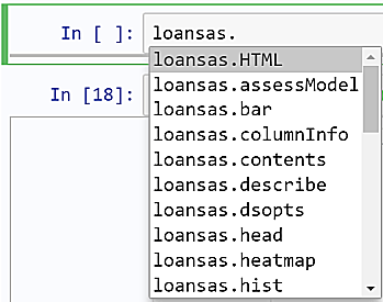
Call the columnInfo method to return column attributes for the loansas object.
loansas.columnInfo()
                The CONTENTS Procedure
    Alphabetic List of Variables and Attributes
#    Variable    Type    Len


15   dti       Num       8
9    emp_len   Char      9
7    grade     Char      1
1    id        Num       8
11   income    Num       8
3    ln_amt    Num       8
12   ln_stat   Char     18
6    m_pay     Num       8
2    mem_id    Num       8
10   own_rnt   Char      8
13   purpose   Char     18
5    rate      Char      6
14   state     Char      2
8    sub_grd   Char      2
4    term      Char     10
From a Jupyter notebook cell display a histogram calling the bar method.
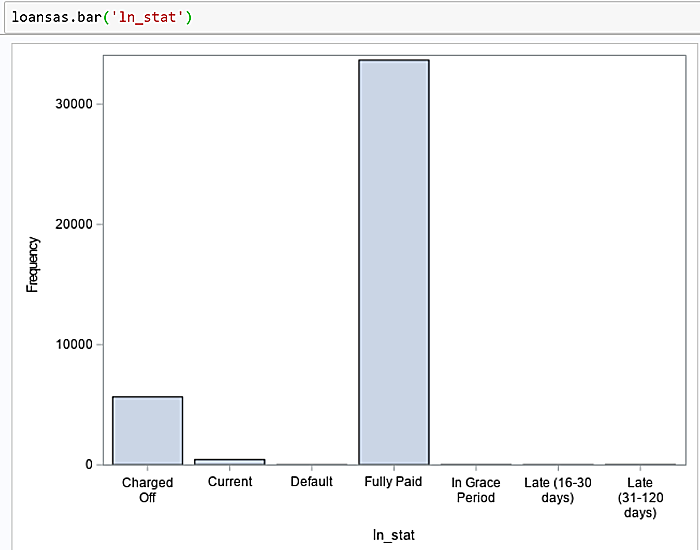
The histogram shows approximately 5,000 loans are charged off, meaning the customer defaulted. Since there are 39,786 rows in the dataset it represents a charge-off rate of roughly 12.6%.
During development for calling into the SASPy module access to the SAS log.
print(sas.saslog())
41956      ;*';*";*/;
41957      data _null_; e = exist('sas_data.loan_ds');
41958      v = exist('sas_data.loan_ds', 'VIEW');
41959       if e or v then e = 1;
41960      te='TABLE_EXISTS='; put te e;run;

TABLE_EXISTS= 1
NOTE: DATA statement used (Total process time):
      real time           0.03 seconds
      cpu time            0.00 seconds


41961
41962
41963      ;*';*";*/;
41964      %put E3969440A681A2408885998500000007;
E3969440A681A2408885998500000007
41965
10                                                                                                                       The SAS System                                                                                              09:04 Friday, June 14, 2019

41966      ;*';*";*/;
41967      data _null_; e = exist('sas_data.loan_ds');
41968      v = exist('sas_data.loan_ds', 'VIEW');
41969       if e or v then e = 1;
41970      te='TABLE_EXISTS='; put te e;run;

TABLE_EXISTS= 1
Call the teach_me_SAS method to return the generated SAS code.
sas.teach_me_SAS(True)
loansas.bar('ln_stat')
sas.teach_me_SAS(False)
proc sgplot data=sas_data.loan_ds;
        vbar ln_stat;
run;
title;
Execute SAS Code
The saspy.SASsession object has the submit method enabling execution of arbitrary blocks of SAS code and returns a dictionary containing the SAS log and any output where ‘LOG’ and ‘LST’ are the keys respectively. The sas_code object uses three quotes ''' to mark the begin and end of the DocString.
sas_code='''
options nodate nonumber;
proc print data=sas_data.loan_ds (obs=5);
   var id;
run;
'''
results = sas.submit(sas_code, results='TEXT')
print(results['LST'])
The SAS System

    Obs      id
      1    872482
      2    872482
      3    878770
      4    878701
      5    878693
The 'LOG' key for the results Dictionary returns the section of the SAS log (rather than the entire log) associated with the block of submitted code.
print(results['LOG'])
41977      options nodate nonumber;
41978      proc print data=sas_data.loan_ds (obs=5);
41979      var id;
41980      run;

NOTE: There were 5 observations read from the data set SAS_DATA.LOAN_DS.
NOTE: The PROCEDURE PRINT printed page 1.
Render SAS output (the listing file) with HTML from a Jupyter notebook.
from IPython.display import HTML
results = sas.submit(sas_code, results='HTML')
HTML(results['LST'])

Write SAS Dataset to DataFrame
SASPy provides the sasdata2dataframe method to write SAS datasets to pandas Dataframes with an alias of sas.sd2df. The sd2df method offers numerous possibilities since a SAS dataset is itself a logical reference mapped to any number of physical data sources. Depending on which products you license a SAS dataset can refer to SAS datasets on a local file system, on a remote file system, SAS/Access Views attached to RDBMS tables, SAS Views, files, and so on.
The sd2df method has five parameters.
- table, the name of the SAS dataset to export to a target DataFrame
- libref, the LIBREF for the SAS dataset
- dsopts, a dictionary containing the following SAS dataset options:
a. WHERE clause
b. KEEP list
c. DROP list
d. OBS
e. FIRSTOBS
f. FORMAT
-
method. The default is MEMORY. If the SAS dataset is large you may get better performance using the CSV method.
-
kwargs, indicating the sd2df method can accept any number of valid parameters passed to it.
Export the SAS Dataset SASHELP.CARS where make = 'Ford' to the cars_df DataFrame.
ds_options = {'where'   : 'make = "Ford"',
              'keep'    : ['msrp enginesize Cylinders Horsepower Make'],
             }

cars_df = sas.sd2df(table='cars', libref='sashelp', dsopts=ds_options, method='CSV')

cars_df.head()
   Make   MSRP  EngineSize  Cylinders  Horsepower
0  Ford  41475         6.8         10         310
1  Ford  34560         4.6          8         232
2  Ford  29670         4.0          6         210
3  Ford  22515         3.0          6         201
4  Ford  13270         2.0          4         130
Illustrate a pipeline integrating SAS and Python logic in a single script with following steps.
1. Use SAS to perform an aggregation on the SAS dataset in.loan_ds calling the submit method.
2. Export the SAS dataset to the grade_sum Dataframe.
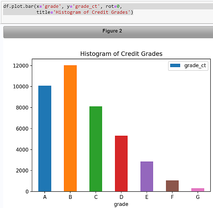
3. Call the pandas plot.bar method to create a histogram of credit risk grades.
sascode='''libname sas_data "c:\data";
proc sql;
   create table grade_sum as
      select grade
           , count(*) as grade_ct
      from sas_data.loan_ds
   group by grade;
quit;'''

run_sas = sas.submit(sascode, results='TEXT')

df = sas.sd2df('grade_sum')
df.head(10)
  grade  grade_ct
0     A     10086
1     B     12029
2     C      8114
3     D      5328
4     E      2857
5     F      1054
6     G       318
df.plot.bar(x='grade', y='grade_ct', rot=0,
           title='Histogram of Credit Grades')
Pass MACRO Variables to Python Objects
The SASPy SASsession object has two methods for passing values. The symget method assigns the value of a SAS Macro variable to a Python object using the syntax:
py_obj = sas.symget(existing_sas_macro_var)
The symput method passes the value of a Python object to a SAS Macro variable value using the syntax:
sas.symput(sas_macro_variable, py_obj)
Illustrate the symget method passing Macro variable values to Python Objects.
The sas_code Doc-string is passed to the submit method for execution. For the Data Step the value from the automatic SAS Macro variable &syserr is assigned to the Macro variable &step1_rc. Similarly, in the PROC step &syserr is assigned to the SAS Macro variable &step2_rc. &syserr is an automatic, read-only Macro variable containing the execution return code from the Data Step and most PROC steps.
sas_code='''data _null_;
   yes = exist('sashelp.class');
   if yes  = 1 then put
      'Table Exists';
    else put
       'Table Does NOT Exist';
    %let step1_rc = &syserr;
run;

proc summary data=sashelp.class;
   var weight;
run;
%let step2_rc = &syserr;
'''
run_sas = sas.submit(sas_code, results='TEXT')

rc = []
rc.append(sas.symget('step1_rc'))
rc.append(sas.symget('step2_rc'))
for i, value in enumerate(rc):
   if value==0:
      print ("Normal Run for Step {}.".format(i, value))
   else:
      print("Abnormal Run for Step {}. RC={}".format(i, value))
Normal Run for Step 0.
Abnormal Run for Step 1. RC=1012
Fetch the SAS log.
print(run_sas[('LOG')])
Which returns:
42032      proc summary data=sashelp.class;
42033         var weight;
42034      run;

ERROR: Neither the PRINT option nor a valid output statement has been given.
NOTE: The SAS System stopped processing this step because of errors.
NOTE: PROCEDURE SUMMARY used (Total process time):
      real time           0.00 seconds
      cpu time            0.00 seconds

42035      %let step2_rc = &syserr;
Pass Python Objects to MACRO Variables
Illustrate the symput method.
py_str="Python and SAS Together"

sas.symput('str_from_py', py_str)
sas_code='''data _null_;
   %put Python passed in: ===> &str_from_py;
'''
run_sas = sas.submit(sas_code, results='TEXT')
print(run_sas[('LOG')])
Fetch the SAS log.
print(run_sas[('LOG')])
42086      data _null_;
42087         %put Python passed in: ===> &str_from_py;
Python passed in: ===> Python and SAS Together
Return the entire SAS log with:
print(sas.saslog())
Prompting
SASPy supports interactive prompting. The first type of prompting is implicit. When running the SASsession method if required arguments to the connection method are not specified in the SAScfg_personal.py configuration file the connection process is halted and the user is prompted for the missing argument(s).
The second form is explicit, meaning the application builder controls how prompts are displayed and processed. Both the submit method and the saslib method accept an additional prompt argument. Prompt arguments are presented at run time connected to SAS Macro variables supplied directly in the SAS code or as arguments to the method calls.
Prompt arguments are supplied as a Python dictionary. Keys are the SAS Macro variable names and values are the Boolean values True or False. Users are prompted for key values and entered values are passed to the Macro variable. The Macro variable name is taken from the dictionary key.
At SAS run time, the Macro variables are resolved. If False is specified as the value for the key/value pair, then users sees the input value entered into the prompt area. On the SAS Log user-entered values are rendered in clear text. If True is specified for the value for the key/value pair then the user does not see the input values; nor is the Macro variable value rendered on the SAS Log.
Illustrate SASPy Prompting.
sas.saslib('sqlsrvr', engine='odbc',
           options='user=&user pw=&pw datasrc=AdventureWorksDW',
           prompt={'user' : False, 'pw': True})
Please enter value for macro variable user Randy
Please enter value for macro variable pw
                                                                                                                        The SAS System

42093
42094      options nosource nonotes;
42097      %let user=Randy;
42098      libname sqlsrvr odbc user=&user pw=&pw datasrc=AdventureWorksDW;
NOTE: Libref SQLSRVR was successfully assigned as follows:
      Engine:        ODBC
      Physical Name: AdventureWorksDW
42099      options nosource nonotes;
The %let assignment for user= is displayed in the log but not for pw=.
Scripting SASPy
The examples above are executed interactively writing output to the Python console or in a Jupyter notebook. SASPy provisions the <a href="https://sassoftware.github.io/saspy/api.html#saspy.SASsession.set_batch"set_batch method to automate Python script execution making calls into SASPy. Mostly from the above examples this script will:
1. Creates the loandf DataFrame calling the read_csv method.
2. Prepare the rate and month columns for mathematical manipulations.
3. Call the saslib method to expose the SAS libref to the Python environment.
4. Call the df2sd method converting the loandf DataFrame to the sas_data.loan_ds SAS dataset.
5. Set the SASPy execution mode to batch.
6. Call the SASPy bar method to generate a histogram.
7. Assign the SAS Listing (html source statements) to the object html_out object.
8. Call the Python Standard Library, open, write, and close calls to write the .html source statements held in the html_out object to a file on the filesystem.
#! /usr/bin/python3.6
import pandas as pd
import saspy
url = url = "https://raw.githubusercontent.com/RandyBetancourt/PythonForSASUsers/master/data/LC_Loan_Stats.csv"

loandf = pd.read_csv(url,
    low_memory=False,
    usecols=(0, 1, 2, 3, 4, 5, 6, 7, 8, 9, 10, 12, 13, 15, 16),
    names=('id',
          'mem_id',
          'ln_amt',
          'term',
          'rate',
          'm_pay',
          'grade',
          'sub_grd',
          'emp_len',
          'own_rnt',
          'income',
          'ln_stat',
          'purpose',
          'state',
          'dti'),
    skiprows=1,
    nrows=39786,
    header=None)

loandf['rate'] = loandf.rate.replace('%','',regex=True).astype('float')/100
loandf['term'] = loandf['term'].str.strip('months').astype('float64')

sas = saspy.SASsession(cfgname='winlocal')

sas.saslib('sas_data', 'BASE', 'C:\data')

loansas = sas.df2sd(loandf, table='loan_ds', libref='sas_data')

sas.set_batch(True)
out=loansas.bar('ln_stat', title="Historgram of Loan Status", label='Loan Status')
html_out = out['LST']

f = open('C:\\data\\saspy_batch\\sas_output.html','w')
f.write(html_out)
f.close()
This script is now callable using any number of methods such as a Windows Shell, Powershell, Bash shell, or a being executed by a scheduler. Copy this code to a file, e.g. saspy_set_batch. On Windows or Linux the command to run the script is:
python saspy_set_batch.py
Datetime Handling
Recall from the Dates and Times section SAS and Python use different offsets for internal representation of datetime values. When datetime values are imported and exported between software the process poses risk for corrupting data values.
This example below creates the df_dates DataFrame by using the dictionary contructor method to include the dates column created by calling the date_range method and the rnd_val column by calling the numpy random.randint method between the range of 100 and 1000 as random numbers.
Also included are elementary error handling features. The connection from the SASsession object checks the SASpid attribute returning the process ID for the SAS sub-process. In the event the call to the SASsession method fails an error message is printed and the script is exited at that point. The call to sys.exit method is similar to the SAS ABORT statement with the ABEND argument to halt the SAS job or session. The ABORT statement actions are influenced by whether the SAS script is executed interactively or batch.
Test SASPy Datatime handling by constructing the df_dates DataFrame and display the first 5 rows.
import saspy
import sys
import pandas as pd
import numpy as np
from datetime import datetime, timedelta, date

nl = '\n'
date_today = date.today()
days       = pd.date_range(date_today, date_today + timedelta(20), freq='D')

np.random.seed(seed=123456)
data = np.random.randint(100, high=10000, size=len(days))

df_dates = pd.DataFrame({'dates': days, 'rnd_val': data})
print(df_dates.head(5))
       dates  rnd_val
0 2019-06-17     6309
1 2019-06-18     6990
2 2019-06-19     4694
3 2019-06-20     3221
4 2019-06-21     3740
Connect to SAS and check the returned SASpid attribute for a non-missing value.
sas = saspy.SASsession(cfgname='winlocal', results='Text')

if sas.SASpid == None:
   print('ERROR: saspy Connection Failed',
         nl,
         'Exiting Script')
   sys.exit()

print(nl,
      'saspy Process ID: ', sas.SASpid,
      nl)
Will return something like:
saspy Process ID: 29860
Call the saslib method to define the sas_data LIBREF. Call and display the assigned_librefs method to return available LIBREFs. Check the SYSLIBRC method return code and exit the script on a non-zero value (0). Call the df2sd to export the df_dates DataFrame to the sas_data.df_dates SAS dataset.
sas.saslib('sas_data', 'BASE', 'C:\data')

sas.assigned_librefs()

if sas.SYSLIBRC() != 0:
   print('ERROR: Invalid Libref',
          nl,
         'Exiting Script')
   sys.exit()

py_dates = sas.df2sd(df_dates, table='py_dates', libref='sas_data')
py_dates.head(5)
 Obs    dates                         rnd_val
   1    2019-06-17T00:00:00.000000      6309
   2    2019-06-18T00:00:00.000000      6990
   3    2019-06-19T00:00:00.000000      4694
   4    2019-06-20T00:00:00.000000      3221
   5    2019-06-21T00:00:00.000000      3740
Call the SASPy columnInfo method for the py_dates object which is an interface to PROC CONTENTS. py_dates is a Python objected mapped to the sas_data.df_dates SAS dataset.
py_dates.columnInfo()
The CONTENTS Procedure

Alphabetic List of Variables and Attributes
#    Variable    Type    Len    Format
1    dates       Num       8    E8601DT26.6
2    rnd_val     Num       8
Call the submit method to display the SAS datatime values for the dates variable with the mdyampmW.d format.
sas_code = '''data _null_;
                 set sas_data.py_dates(obs=5);
               put 'Datetime dates: ' dates mdyampm25.;
               run;'''
run_sas = sas.submit(sas_code, results='TEXT')
print(run_sas[('LOG')])
Returns:
134        data _null_;
135                         set sas_data.py_dates(obs=5);
136                       put 'Datetime dates: ' dates mdyampm25.;
137                       run;

Datetime dates:        6/17/2019 12:00 AM
Datetime dates:        6/18/2019 12:00 AM
Datetime dates:        6/19/2019 12:00 AM
Datetime dates:        6/20/2019 12:00 AM
Datetime dates:        6/21/2019 12:00 AM
NOTE: There were 5 observations read from the data set SAS_DATA.PY_DATES.
Now let’s go the other direction and export the sas_data.py_dates dataset to the sasdt_df2 DataFrame.
sasdt_df2 = sas.sd2df(table='py_dates', libref='sas_data')

print(nl,
      sasdt_df2.head(5),
      nl,
      'Data type for date_times:', sasdt_df2['dates'].dtype,
      nl)
Displaying the first 5 rows of the sasdt_df2 DataFrame.
        dates  rnd_val
0 2019-06-17     6309
1 2019-06-18     6990
2 2019-06-19     4694
3 2019-06-20     3221
4 2019-06-21     3740
 Data type for date_times: datetime64[ns]
Construct the new DataFrame column date_times_fmt calling the dt.strftimeto display this column as day, date, time, and year.
sasdt_df2["date_times_fmt"] = sasdt_df2["dates"].dt.strftime("%c")
print(sasdt_df2["date_times_fmt"].head(5))
0    Mon Jun 17 00:00:00 2019
1    Tue Jun 18 00:00:00 2019
2    Wed Jun 19 00:00:00 2019
3    Thu Jun 20 00:00:00 2019
4    Fri Jun 21 00:00:00 2019
The entire script in one go...
import saspy
import sys
import pandas as pd
import numpy as np
from datetime import datetime, timedelta, date

nl = '\n'
date_today = date.today()
days       = pd.date_range(date_today, date_today + timedelta(20), freq='D')

np.random.seed(seed=123456)
data = np.random.randint(100, high=10000, size=len(days))

df_dates = pd.DataFrame({'dates': days, 'rnd_val': data})
print(df_dates.head(5))

sas = saspy.SASsession(cfgname='winlocal', results='Text')

if sas.SASpid == None:
   print('ERROR: saspy Connection Failed',
         nl,
         'Exiting Script')
   sys.exit()

print(nl,
      'saspy Process ID: ', sas.SASpid,
      nl)

sas.saslib('sas_data', 'BASE', 'C:\data')

sas.assigned_librefs()

if sas.SYSLIBRC() != 0:
   print('ERROR: Invalid Libref',
          nl,
         'Exiting Script')
   sys.exit()

py_dates = sas.df2sd(df_dates, table='py_dates', libref='sas_data')
py_dates.head(5)

py_dates.columnInfo()


sas_code = '''data _null_;
                 set sas_data.py_dates(obs=5);
               put 'Datetime dates: ' dates mdyampm25.;
               run;'''
run_sas = sas.submit(sas_code, results='TEXT')
print(run_sas[('LOG')])

sasdt_df2 = sas.sd2df(table='py_dates', libref='sas_data')

print(nl,
      sasdt_df2.head(5),
      nl,
      'Data type for date_times:', sasdt_df2['dates'].dtype,
      nl)

sasdt_df2["date_times_fmt"] = sasdt_df2["dates"].dt.strftime("%c")
print(sasdt_df2["date_times_fmt"].head(5))