Introduction
This section introduces pandas library, whose DataFrame object is similar to a SAS dataset.
| pandas | SAS |
|---|---|
| DataFrame | Dataset |
| Row | Observation |
| Column | Variable |
| GroupBy | By-Group |
| NaN | . (period) |
| Slice | Subset |
Series
Think of a Series as a DataFrame with a single column.
import numpy as np
import pandas as pd
from numpy.random import randn
np.random.seed(54321)
s1 = pd.Series(randn(10))
print(s1.head(5))
0        0.223979
1        0.744591
2       -0.334269
3        1.389172
4       -2.296095
dtype: float64
The SAS analog uses an array. Unlike most other programming languages, a SAS ARRAY is not a data structure. Rather, it is a convenience to iterate over groups of similar variables or values assigned to the array elements.
data _null_;
   call streaminit(54321);

array s2 {10};
   do i = 1 to 10;
      s2{i} = rand("Normal");
      if i <= 5 then put s2{i};
   end;
run;
-1.364866914
1.9696792198
0.5123294653
-0.597981097
-0.895650739
RangeIndex
Rather than using the default RangeIndex object we can assign labels to the rows with an index. See more details in the Indexing section of this site.
import numpy as np
import pandas as pd
from numpy.random import randn
np.random.seed(54321)
s2 = pd.Series(randn(10), index=['a', 'b', 'c', 'd', 'e', 'f', 'g', 'h', 'i', 'j'])
print(s2.head(5))
a    0.223979
b    0.744591
c   -0.334269
d    1.389172
e   -2.296095
dtype: float64
Series elements are returned either by their default index position (using the RangeIndex) or by user-defined index values.
print(s2[0])
0.22397889127879958
print(s2['a'])
0.22397889127879958
SAS arrays must use a non-zero index start position for element retrieval.
data _null_;
   call streaminit(54321);

array s2 {10} ;
   do i = 1 to 10;
      s2{i} = rand("Normal");
      if i = 1 then put s2{i};
   end;
run;
-1.364866914
Retrieval of values from a Series follows the string-slicing pattern presented in the string slicing section. The value to the left of the colon (:) separator is the start position for the Series’ index location and values to the right identify the stop position for the element location.
print(s2[:3])
a    0.223979
b    0.744591
c   -0.334269
dtype: float64
print(s2[:'c'])
a    0.223979
b    0.744591
c   -0.334269
dtype: float64
Returning the first three elements in a SAS ARRAY.
data _null_;
   call streaminit(54321);

array s2 {10} ;
   do i = 1 to 10;
      s2{i} = rand("Uniform");
      if i <= 3 then put s2{i};
   end;
run;
0.4322317771
0.5977982974
0.7785986471
A Series allows mathematical operations to be combined with Boolean comparisons as a condition for returning elements.
s2[s2 < s2.mean()]
2   -0.334269
4   -2.296095
7   -0.082760
8   -0.651688
9   -0.016022
dtype: float64
DataFrames
Think of a pandas DataFrame as a collection of Series into a relational-like structure with labels. There are numerous constructor methods for creating DataFrames.
We illustrate the read_csv constructor method. The original data is made public by the UK government's Accident Report Data from the year 2015. A copy of the data is stored here on Github.
file_loc = "https://raw.githubusercontent.com/RandyBetancourt/PythonForSASUsers/master/data/uk_accidents.csv"
df = pd.read_csv(file_loc)
print(df.shape)
(266776, 27)
The shape attribute shows the df DataFrame has 266,776 rows and 27 columns.
Use PROC IMPORT to read the same .csv file into a SAS dataset.
filename git_csv temp;
proc http
   url="https://raw.githubusercontent.com/RandyBetancourt/PythonForSASUsers/master/data/uk_accidents.csv"
   method="GET"
   out=git_csv;

proc import datafile = git_csv
      dbms=csv
      out=uk_accidents;
run;
NOTE: 266776 records were read from the infile GIT_CSV.
      The minimum record length was 65.
      The maximum record length was 77.
NOTE: The data set WORK.UK_ACCIDENTS has 266776 observations and 27 variables.

266776 rows created in WORK.UK_ACCIDENTS from GIT_CSV.

NOTE: WORK.UK_ACCIDENTS data set was successfully created.
DataFrame Validation
pandas provide a number of methods for data validation. In this example, the info function is similar to PROC CONTENTS.
print(df.info())
<class 'pandas.core.frame.DataFrame'>
RangeIndex: 266776 entries, 0 to 266775
Data columns (total 27 columns):
Accident_Severity               266776 non-null int64
Number_of_Vehicles              266776 non-null int64
Number_of_Casualties            266776 non-null int64
Day_of_Week                     266776 non-null int64
Time                            266752 non-null object
Road_Type                       266776 non-null int64
Speed_limit                     266776 non-null int64
Junction_Detail                 266776 non-null int64
Light_Conditions                266776 non-null int64
Weather_Conditions              266776 non-null int64
Road_Surface_Conditions         266776 non-null int64
Urban_or_Rural_Area             266776 non-null int64
Vehicle_Reference               266776 non-null int64
Vehicle_Type                    266776 non-null int64
Skidding_and_Overturning        266776 non-null int64
Was_Vehicle_Left_Hand_Drive_    266776 non-null int64
Sex_of_Driver                   266776 non-null int64
Age_of_Driver                   266776 non-null int64
Engine_Capacity__CC_            266776 non-null int64
Propulsion_Code                 266776 non-null int64
Age_of_Vehicle                  266776 non-null int64
Casualty_Class                  266776 non-null int64
Sex_of_Casualty                 266776 non-null int64
Age_of_Casualty                 266776 non-null int64
Casualty_Severity               266776 non-null int64
Car_Passenger                   266776 non-null int64
Date                            266776 non-null object
dtypes: int64(25), object(2)
memory usage: 55.0+ MB
The dtype attribute returns the DataFrame column type,
df['Date'].dtype
dtype('O')
indicating the Date column is type 'Object' or a string.
Use the parse_dates= argument to read the Date column as a datetime.
file_loc = "C:\\Data\\uk_accidents.csv"
df = pd.read_csv(file_loc, parse_dates=['Date'])
Note the double backslashes (\\) for normalizing the path name.
DataFrame Inspection
To inspect the last n rows of a DataFrame pass an integer argument to the tail function.
df.tail(10)
Accident_Severity     ...            Date
266766                  2     ...       8/30/2015
266767                  3     ...      11/29/2015
266768                  3     ...      11/29/2015
266769                  3     ...      11/29/2015
266770                  3     ...       7/26/2015
266771                  3     ...       7/26/2015
266772                  3     ...      12/31/2015
266773                  3     ...       7/28/2015
266774                  3     ...       7/28/2015
266775                  3     ...       7/15/2015

[10 rows x 27 columns]
SAS uses FIRSTOBS and OBS dataset options followed by a value for _N_ with most procedures to determine which observations are included for processing.
proc print data = uk_accidents (firstobs = 266767);
   var Accident_Severity Date;
run;
NOTE: There were 10 observations read from the data set WORK.UK_ACCIDENTS.

The head(5) function returns the first 5 rows from a DataFrame.
df.head(5)
   Accident_Severity    ...           Date
0                  3    ...       1/9/2015
1                  3    ...       1/9/2015
2                  3    ...      2/23/2015
3                  3    ...      2/23/2015
4                  3    ...      2/23/2015
To display the first 5 observations in a SAS dataset.
proc print data=uk_accidents (obs = 5);
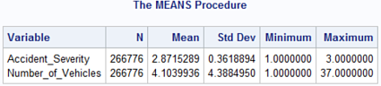
The DataFrame describe function reports measures of central tendencies, dispersion and shape for all numeric types.
df.describe()
df.describe()
       Accident_Severity  Number_of_Vehicles      ...
count      266776.000000       266776.000000      ...
mean            2.871529            4.103994      ...
std             0.361889            4.388495      ...
min             1.000000            1.000000      ...
25%             3.000000            2.000000      ...
50%             3.000000            2.000000      ...
75%             3.000000            3.000000      ...
max             3.000000           37.000000      ...

[8 rows x 25 columns]
PROC MEANS returns output similar to the describe function.
The slicing operator [ ] selects a set of rows and/or columns from a DataFrame. The section on Indexing provides detailed examples of row-slicing (sub-setting).
df[['Sex_of_Driver', 'Time']].head(10)
   Sex_of_Driver   Time
0              1  19:00
1              1  19:00
2              1  18:30
3              2  18:30
4              1  18:30
5              1  17:50
6              1  17:50
7              1   7:05
8              1   7:05
9              1  12:30
The SAS syntax for displaying the first 10 observations for the Sex_of_Driver and Time variables is:
proc print data=uk_accidents (obs = 10);
   var Sex_of_Driver Time;
run;
There are numerous visualization methods for DataFrames to derive meaningful information. One such example is the hist method from the matplotlib library for rendering a histogram.
import matplotlib.pyplot as plt
df.hist(column='Sex_of_Driver', grid=False)
plt.show()
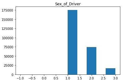
From the supplied metadata we know the Sex_of_Driver column value of 1 maps to Males, 2 to Females, 3 to Not Known and -1 to Data Missing or out of Range. We see males have an accident rate over twice that of females.
Missing Data
pandas use two sentinel values to indicate missing data; the Python None object and NaN (not a number) object. The None object is used as a missing value indicator for DataFrame columns with a type of object (character strings). NaN is a special floating point value indicating missing for float64 columns. See the pandas discussion on missing data here.
Use the DataFrame constructor method to create the df1 DataFrame.
nl = '\n'

df1 = pd.DataFrame([['cold', 9],
                    ['warm', 4],
                    [None  , 4]],
                    columns=['Strings', 'Integers'])
print(nl,
     df1,
     nl,
     df1.dtypes)
  Strings  Integers
0    cold         9
1    warm         4
2    None         4
Strings     object
Integers     int64
dtype: object
The value for the Strings column on row 2 is missing indicated by the None object for its value. If we update the Integers column value of 9 to None, pandas automatically maps the value to a NaN.
df1.loc[df1.Integers == 9, 'Integers'] = None
print(nl,
      df1,
      nl,
      df1.dtypes)
  Strings  Integers
0    cold       NaN
1    warm       4.0
2    None       4.0
Strings      object
Integers    float64
dtype: object
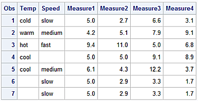
In this example the None object indicates missing for columns with type 'object' (character data) and columns with type float64 (numeric data).
df2 = pd.DataFrame([['cold','slow', None, 2.7, 6.6, 3.1],
                    ['warm', 'medium', 4.2, 5.1, 7.9, 9.1],
                    ['hot', 'fast', 9.4, 11.0, None, 6.8],
                    ['cool', None, None, None, 9.1, 8.9],
                    ['cool', 'medium', 6.1, 4.3, 12.2, 3.7],
                    [None, 'slow', None, 2.9, 3.3, 1.7],
                    [None, 'slow', None, 2.9, 3.3, 1.7]],
                    columns=['Temp', 'Speed', 'Measure1', 'Measure2', 'Measure3', 'Measure4'])
print(nl,
      df2,
      nl)
   Temp   Speed  Measure1  Measure2  Measure3  Measure4
0  cold    slow       NaN       2.7       6.6       3.1
1  warm  medium       4.2       5.1       7.9       9.1
2   hot    fast       9.4      11.0       NaN       6.8
3  cool    None       NaN       NaN       9.1       8.9
4  cool  medium       6.1       4.3      12.2       3.7
5  None    slow       NaN       2.9       3.3       1.7
6  None    slow       NaN       2.9       3.3       1.7
Print the column types.
print(df2.dtypes)
Temp         object
Speed        object
Measure1    float64
Measure2    float64
Measure3    float64
Measure4    float64
dtype: object
Detect Missing Values
Below is the list the functions applied to a pandas DataFrame or Series to detect and replace missing values.
| Function | Action Taken |
|---|---|
| isnull | Generates a Boolean mask indicating missing values |
| notnull | Opposite of isnull |
| dropna | Returns a filtered copy of the original DataFrame |
| fillna | Returns a copy of the original DataFrame with missing values filled or imputed |
One approach for locating missing values in a DataFrame is to iterate along all of the columns with a for statement.
for col_name in df2.columns:
     print (col_name, end="---->")
     print (sum(df2[col_name].isnull()))
Temp---->2
Speed---->1
Measure1---->4
Measure2---->1
Measure3---->1
Measure4---->0
It turns out this approach is sub-optimal since we can apply isnull to the DataFrame rather than the columns.
df2.isnull().sum()
Temp        2
Speed       1
Measure1    4
Measure2    1
Measure3    1
Measure4    0
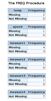
For SAS, one approach is the create a user-defined format for numeric and character variables and then use them in a call to PROC FREQ to identify variables with missing values.
data df;
   infile cards;
   input temp $4.
         speed $7.
     @14 measure1
     @18 measure2
     @23 measure3
     @28 measure4 ;
list;
datalines;
cold slow    .   2.7  6.6  3.1
warm medium  4.2 5.1  7.9  9.1
hot  fast    9.4 11.0 .    6.8
cool         .   .    9.1  8.9
cool medium  6.1 4.3  12.2 3.7
     slow    .   2.9  3.3  1.7
     slow    .   2.9  3.3  1.7
;;;;
proc print data =df;
run;

proc format;
   value $missfmt ' '='Missing' other='Not Missing';

   value  missfmt  . ='Missing' other='Not Missing';

proc freq data=df;
   format _CHARACTER_ $missfmt.;
   tables _CHARACTER_ / missing missprint nocum nopercent;

   format _NUMERIC_ missfmt.;
   tables _NUMERIC_ / missing missprint nocum nopercent;
run;
The MISSING option for the TABLES statement is required in order for PROC FREQ to include missing values in its output.
The isnull method creates a Boolean mask by returning a DataFrame of Boolean values.
print(df2)
   Temp   Speed  Measure1  Measure2  Measure3  Measure4
0  cold    slow       NaN       2.7       6.6       3.1
1  warm  medium       4.2       5.1       7.9       9.1
2   hot    fast       9.4      11.0       NaN       6.8
3  cool    None       NaN       NaN       9.1       8.9
4  cool  medium       6.1       4.3      12.2       3.7
5  None    slow       NaN       2.9       3.3       1.7
6  None    slow       NaN       2.9       3.3       1.7
df2.isnull()
    Temp  Speed  Measure1  Measure2  Measure3  Measure4
0  False  False      True     False     False     False
1  False  False     False     False     False     False
2  False  False     False     False      True     False
3  False   True      True      True     False     False
4  False  False     False     False     False     False
5   True  False      True     False     False     False
6   True  False      True     False     False     False
The isnull method returns a DataFrame of Boolean values with None objects and NaN’s returned as True and non-missing values returned as False.
The notnull method is the inverse of the isnull method. It produces a Boolean mask where null or missing values are returned as False and non-missing values are returned as True.
The behavior of missing values for DataFrames used in mathematical operations and functions is similar to SAS’ behavior. In the case of DataFrames:
-
Row-wise operations on missing data propagate missing values.
-
Methods and function missing values are treated as zero.
-
If all data values are missing, the results from methods and functions will be 0 (zero).
df2['Sum_M3_M4'] = df2['Measure3'] + df2['Measure4']
print(df2[['Measure3', 'Measure4', 'Sum_M3_M4']])
Measure3  Measure4  Sum_M3_M4
0       6.6       3.1        9.7
1       7.9       9.1       17.0
2       NaN       6.8        NaN
3       9.1       8.9       18.0
4      12.2       3.7       15.9
5       3.3       1.7        5.0
6       3.3       1.7        5.0
In a row-wise arithmetic operation NaNs are proprogated. Notice the print method displays a subset of columns from df2 DataFrame. The syntax:
print(df2[['Measure3', 'Measure4', 'Sum_M3_M4']])
is a form of DataFrame slicing using the [ ] operator to slice the columns Measure3, Measure4, and Sum_M3_M4 passed to the print method. See the Slice Rows by Position section for detailed examples.
The SAS analog:
proc print data=df2;
   var measure3 measure4 sum_m3_m4;
run;
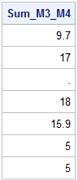
Below, the sum method is applied to the column Sum_M3_M4 resulting in the NaN mapped to zero (0).
print(df2[['Sum_M3_M4']])
   Sum_M3_M4
0        9.7
1       17.0
2        NaN
3       18.0
4       15.9
5        5.0
6        5.0
df2['Sum_M3_M4'].sum()
70.6
In the following SAS example, the SUM function behaves the same way.
proc sql;
   create table df_sum as
   select *
       , (measure3 + measure4) as Sum_M3_M4
   from df;

   select Sum_M3_M4
   from df_sum;

   select 'Sum Function Applied to Measure 5'
          ,sum(Sum_M3_M4)
    from df_sum;
quit;
NOTE: Table WORK.DF_SUM created, with 7 rows and 7 columns.

If you want to override the pandas' behavior in cases where it maps NaN's to zero, use the skipna=False argument.
print(df2[['Sum_M3_M4']])
   Sum_M3_M4
0        9.7
1       17.0
2        NaN
3       18.0
4       15.9
5        5.0
6        5.0
df2['Sum_M3_M4'].sum(skipna=False)
nan
Applying the pandas sum method to a column with all missing values returns zero.
df2['Measure5'] = None
print(df2['Measure5'])
0    None
1    None
2    None
3    None
4    None
5    None
6    None
Name: Measure5, dtype: object
df2['Measure5'].sum()
0
With SAS, the SUM function returns missing if all variables values are missing and returns 0 (zero) when summing zero (0) with all missing values.
data _null_;
   do i= 1 to 7;
      measure5 = .;
      put measure5;
      sum_m5 = sum(measure5);
      sum_0_m5 = sum(0, measure5);
   end;

put 'SUM(measure5) Returns:' sum_m5;
put 'SUM(0, measure5) Returns:' sum_0_m5;
run;
.
.
.
.
.
.
.
SUM(measure5) Returns:.
SUM(0, measure5) Returns:0
Drop Missing Values
Calling the dropna method without a parameter drops rows where one or more values are missing regardless of the column’s type. The default behavior is to operate along rows, or axis 0 and return a copied DataFrame. The default inplace=False argument can be set to True in order to perform an in-place update.
df3=df2.dropna()
print(df3)
   Temp   Speed  Measure1  Measure2  Measure3  Measure4
1  warm  medium       4.2       5.1       7.9       9.1
4  cool  medium       6.1       4.3      12.2       3.7
Unlike the example above, the example below does not create a new DataFrame.
df4 = pd.DataFrame([['cold','slow', None, 2.7, 6.6, 3.1],
                  ['warm', 'medium', 4.2, 5.1, 7.9, 9.1],
                  ['hot', 'fast', 9.4, 11.0, None, 6.8],
                  ['cool', None, None, None, 9.1, 8.9],
                  ['cool', 'medium', 6.1, 4.3, 12.2, 3.7],
                  [None, 'slow', None, 2.9, 3.3, 1.7],
                  [None, 'slow', None, 2.9, 3.3, 1.7]],
                  columns=['Temp', 'Speed', 'Measure1',
                  'Measure2', 'Measure3', 'Measure4'])
print(df4)
   Temp   Speed  Measure1  Measure2  Measure3  Measure4
0  cold    slow       NaN       2.7       6.6       3.1
1  warm  medium       4.2       5.1       7.9       9.1
2   hot    fast       9.4      11.0       NaN       6.8
3  cool    None       NaN       NaN       9.1       8.9
4  cool  medium       6.1       4.3      12.2       3.7
5  None    slow       NaN       2.9       3.3       1.7
6  None    slow       NaN       2.9       3.3       1.7
Instead, the original df4 DataFrame is updated in place.
df4.dropna(inplace=True)
print(df4)
   Temp   Speed  Measure1  Measure2  Measure3  Measure4
1  warm  medium       4.2       5.1       7.9       9.1
4  cool  medium       6.1       4.3      12.2       3.7
The SAS CMISS function is used to detect and then delete observations with one or more missing values.
data df4;
   set df;
   if cmiss(of _all_) then delete;

proc print data = df4;
run;
NOTE: There were 7 observations read from the data set WORK.DF.
NOTE: The data set WORK.DF4 has 2 observations and 6 variables.
The argument to the CMISS function uses the automatic SAS variable _N_ to designate all variables in the dataset.

The dropna method works along a column axis. DataFrames refer to rows as axis 0 and columns as axis 1. The default behavior for the dropna method is to operate along axis 0.
print(df2)
   Temp   Speed  Measure1  Measure2  Measure3  Measure4
0  cold    slow       NaN       2.7       6.6       3.1
1  warm  medium       4.2       5.1       7.9       9.1
2   hot    fast       9.4      11.0       NaN       6.8
3  cool    None       NaN       NaN       9.1       8.9
4  cool  medium       6.1       4.3      12.2       3.7
5  None    slow       NaN       2.9       3.3       1.7
6  None    slow       NaN       2.9       3.3       1.7
df2.dropna(axis=1)
   Measure4
0       3.1
1       9.1
2       6.8
3       8.9
4       3.7
5       1.7
6       1.7
To perform the same action in SAS, an approach is:
- Create an ODS OUTPUT table with the NLEVELS option for PROC FREQ to identify variables containing missing values.
- Create the Macro variable &drop with PROC SQL; SELECT INTO : and the FROM clause referring to the ODS ouput table.
- Create the output df2 dataset with a DROP list formed with the &drop Macro variable.
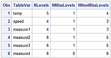
ods output nlevels=nlvs;
proc freq data=df nlevels;
tables _all_;
ods select nlevels;
proc print data=nlvs;
run;
proc sql noprint ;
select tablevar into :drop separated by ' '
from nlvs
where NMissLevels ne 0;
quit;
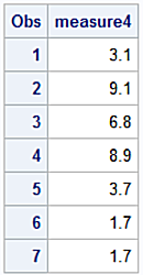
data df2;
set df(drop=&drop);
run;
proc print data=df2;
run;
Output for the WORK.NLVS dataset.
Output for the df2 dataset.
Duplicate Rows
Create the df6 DataFrame by applying the drop_duplicates attribute to the df2 DataFrame. In DataFrame df2 rows 5 and 6 are identical. The section on data management describes additional strategies for finding and updating duplicate values,
df6 = df2.drop_duplicates()
print(df6)
   Temp   Speed  Measure1  Measure2  Measure3  Measure4
0  cold    slow       NaN       2.7       6.6       3.1
1  warm  medium       4.2       5.1       7.9       9.1
2   hot    fast       9.4      11.0       NaN       6.8
3  cool    None       NaN       NaN       9.1       8.9
4  cool  medium       6.1       4.3      12.2       3.7
5  None    slow       NaN       2.9       3.3       1.7
The NODUPRECS option identifies observations with identical values for all variables and removes from the output data set.
proc sort data = df
     out = df6
     noduprecs;
by measure1;
run;

proc print data=df6;
run;
NOTE: 1 duplicate observation were found
The examples using the dropna method drop a fair amount of ‘good’ data. Rather than dropping the entire a row or column if a missing value is encountered the thresh= parameter specifies a minimum number of non-missing values for a row or column to be kept when dropping missing values.
print(df2)
   Temp   Speed  Measure1  Measure2  Measure3  Measure4
0  cold    slow       NaN       2.7       6.6       3.1
1  warm  medium       4.2       5.1       7.9       9.1
2   hot    fast       9.4      11.0       NaN       6.8
3  cool    None       NaN       NaN       9.1       8.9
4  cool  medium       6.1       4.3      12.2       3.7
5  None    slow       NaN       2.9       3.3       1.7
6  None    slow       NaN       2.9       3.3       1.7
df7 = df2.dropna(thresh=4)
print(df7)
   Temp   Speed  Measure1  Measure2  Measure3  Measure4
0  cold    slow       NaN       2.7       6.6       3.1
1  warm  medium       4.2       5.1       7.9       9.1
2   hot    fast       9.4      11.0       NaN       6.8
4  cool  medium       6.1       4.3      12.2       3.7
5  None    slow       NaN       2.9       3.3       1.7
6  None    slow       NaN       2.9       3.3       1.7
The thresh=4 parameter iterates through the rows keeping rows having at least four non-missing values. Row 3 is dropped since it contains only 3 non-missing values.
Instead of dropping entire rows or columns, missing values can imputed using mathematical and statistical functions. The fillna method returns a Series or DataFrame by replacing missing values with derived values.
print(df2)
   Temp   Speed  Measure1  Measure2  Measure3  Measure4
0  cold    slow       NaN       2.7       6.6       3.1
1  warm  medium       4.2       5.1       7.9       9.1
2   hot    fast       9.4      11.0       NaN       6.8
3  cool    None       NaN       NaN       9.1       8.9
4  cool  medium       6.1       4.3      12.2       3.7
5  None    slow       NaN       2.9       3.3       1.7
6  None    slow       NaN       2.9       3.3       1.7
df8 = df2.fillna(0)
print(df8)
   Temp   Speed  Measure1  Measure2  Measure3  Measure4
0  cold    slow       0.0       2.7       6.6       3.1
1  warm  medium       4.2       5.1       7.9       9.1
2   hot    fast       9.4      11.0       0.0       6.8
3  cool       0       0.0       0.0       9.1       8.9
4  cool  medium       6.1       4.3      12.2       3.7
5     0    slow       0.0       2.9       3.3       1.7
6     0    slow       0.0       2.9       3.3       1.7
The fillna method accepts a dictionary of values as a argument. A dictionary is as a collection of key/value pairs where keys are unique within the dictionary. A pair of braces creates an empty dictionary: { }. Placing a comma-separated list of key:value pairs within the braces adds keys:values to the dictionary.
df10 = df2.fillna({
    'Temp'  : 'cold',
    'Speed' : 'slow',
    'Measure1' : 0,
    'Measure2' : 0,
    'Measure3' : 0,
    'Measure4' : 0,
})
print(df10)
   Temp   Speed  Measure1  Measure2  Measure3  Measure4
0  cold    slow       0.0       2.7       6.6       3.1
1  warm  medium       4.2       5.1       7.9       9.1
2   hot    fast       9.4      11.0       0.0       6.8
3  cool    slow       0.0       0.0       9.1       8.9
4  cool  medium       6.1       4.3      12.2       3.7
5  cold    slow       0.0       2.9       3.3       1.7
6  cold    slow       0.0       2.9       3.3       1.7
Another imputation method is replacing NaN’s with the arithmetic mean from a column having few or no missing values. This assumes the columns have nearly equal measures of dispersion.
print(df2)
   Temp   Speed  Measure1  Measure2  Measure3  Measure4
0  cold    slow       NaN       2.7       6.6       3.1
1  warm  medium       4.2       5.1       7.9       9.1
2   hot    fast       9.4      11.0       NaN       6.8
3  cool    None       NaN       NaN       9.1       8.9
4  cool  medium       6.1       4.3      12.2       3.7
5  None    slow       NaN       2.9       3.3       1.7
6  None    slow       NaN       2.9       3.3       1.7
df11 = df2[["Measure1", "Measure2", "Measure3"]].fillna(df2.Measure4.mean())
print(df11)
   Measure1  Measure2  Measure3
0       5.0       2.7       6.6
1       4.2       5.1       7.9
2       9.4      11.0       5.0
3       5.0       5.0       9.1
4       6.1       4.3      12.2
5       5.0       2.9       3.3
6       5.0       2.9       3.3
The same approach with SAS.
data df2;
   infile cards dlm=',';
   input Temp $
          Speed $
          Measure1
          Measure2
          Measure3
          Measure4 ;
list;
datalines;
cold, slow, ., 2.7, 6.6, 3.1
warm, medium, 4.2, 5.1, 7.9, 9.1
hot, fast, 9.4, 11.0, ., 6.8
cool, , ., ., 9.1, 8.9
cool, medium, 6.1, 4.3, 12.2, 3.7
 , slow, ., 2.9, 3.3, 1.7
 , slow, ., 2.9, 3.3, 1.7
;;;;
run;
   proc sql norpint;
     select mean(Measure4) into :M4_mean
   from df2;
quit;

data df11(drop=i);
   set df2;
   array x {3} Measure1-Measure3;
do i = 1 to 3;
  if x(i) = . then x(i) = &M4_mean;
end;
format Measure1-Measure4 8.1;

proc print data=df11;
run;