Introduction
In this section we cover panda readers for .csv files, xls files, http pages, JSON, RDBMS tables and queries along with their writer counterparts. pandas readers and writers are a collection of input/output methods for writing and loading/extracting values into DataFrames. These input/output methods are analogous to the family of SAS/Access Software used to read data values into SAS datasets and write SAS datasets into target output formats.
Reader methods have arguments to specify:
• Input and output locations
• Column and index location and names
• Parsing rules for handling incoming data
• Missing data rules
• Datetime handling
• Quoting rules
• Compression and file formats
• Error handling
Read .csv
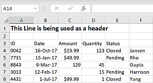
Read the following .csv file calling the read_csv method.
import pandas as pd
url = "https://raw.githubusercontent.com/RandyBetancourt/PythonForSASUsers/master/data/messy_input.csv"

df1 = pd.read_csv(url, skiprows=2)
print(df1)
     ID       Date   Amount  Quantity   Status Unnamed: 5
0    42  16-Oct-17  $23.99      123.0   Closed     Jansen
1  7731  15-Jan-17  $49.99        NaN  Pending        Rho
2  8843   9-Mar-17      129      45.0      NaN      Gupta
3  3013  12-Feb-17               15.0  Pending   Harrison
4  4431   1-Jul-17  $99.99        1.0   Closed       Yang
Print the column types.
print(df1.dtypes)
ID              int64
Date           object
Amount         object
Quantity      float64
Status         object
Unnamed: 5     object
dtype: object
Use the na_values= argument to represent missing for both character and numeric column types.
miss = {'Amount' : [' ', 'NA']}
df2 = pd.read_csv(url, skiprows=2, na_values=miss)
print(df2)
     ID       Date   Amount  Quantity   Status Unnamed: 5
0    42  16-Oct-17  $23.99      123.0   Closed     Jansen
1  7731  15-Jan-17  $49.99        NaN  Pending        Rho
2  8843   9-Mar-17      129      45.0      NaN      Gupta
3  3013  12-Feb-17      NaN      15.0  Pending   Harrison
4  4431   1-Jul-17  $99.99        1.0   Closed       Yang
Before.
df1[3:4]
     ID       Date Amount  Quantity   Status Unnamed: 5
3  3013  12-Feb-17             15.0  Pending   Harrison
After.
df2[3:4]
     ID       Date Amount  Quantity   Status Unnamed: 5
3  3013  12-Feb-17    NaN      15.0  Pending   Harrison
The read_csv reader has two parameters to set column types; the dtype= and the converters= arguments. Both accept dictionary key/value pairs with keys identifying target columns and values that are functions converting values into their corresponding column type.
The dtype= argument allows specification on treating incoming values, for example, either as strings or numeric types. The converter= argument allows calling conversion functions mapping data into the desired column type.
For example, parsing a string value to be read as a datetime. The converters= argument takes precedence over the dtype= argument in the event both are used together.
Illustrates the dtype= argument to map the ID column type to object.
df3 = pd.read_csv(url, skiprows=2, na_values=miss, dtype={'ID' : object})
print(df3)
     ID       Date   Amount  Quantity   Status Unnamed: 5
0  0042  16-Oct-17  $23.99      123.0   Closed     Jansen
1  7731  15-Jan-17  $49.99        NaN  Pending        Rho
2  8843   9-Mar-17      129      45.0      NaN      Gupta
3  3013  12-Feb-17      NaN      15.0  Pending   Harrison
4  4431   1-Jul-17  $99.99        1.0   Closed       Yang
Before.
print(df2['ID'].dtype)
int64
After.
print(df3['ID'].dtype)
object
Illustrate the converters= argument.
Define the strip_sign function to remove dollar signs ($) from incoming values for the Amount column. The converters= argument uses the dictionary key/value pair with the key identifying the Amount column and the corresponding value naming the converter function, in this case, strip_sign.
import math

def strip_sign(x):
        y = x.strip()
        if not y:
            return math.nan
        else:
            if y[0] == '$':
               return float(y[1:])
            else:
                return float(y)

df4 = pd.read_csv(url, skiprows=2, converters={'ID' : str, 'Amount': strip_sign})

print(df4,
      '\n', '\n',
      'Amount dtype:', df4['Amount'].dtype)
     ID       Date  Amount  Quantity   Status Unnamed: 5
0  0042  16-Oct-17   23.99     123.0   Closed     Jansen
1  7731  15-Jan-17   49.99       NaN  Pending        Rho
2  8843   9-Mar-17  129.00      45.0      NaN      Gupta
3  3013  12-Feb-17     NaN      15.0  Pending   Harrison
4  4431   1-Jul-17   99.99       1.0   Closed       Yang

 Amount dtype: float64
Illustrate mapping the ID column as a string and set it as the DataFrame index at the end of the read/parse operation.
df5 = pd.read_csv(url, skiprows=2, na_values=miss, converters={'ID' : str}).set_index('ID')
print(df5)
           Date   Amount  Quantity   Status Unnamed: 5
ID
0042  16-Oct-17  $23.99      123.0   Closed     Jansen
7731  15-Jan-17  $49.99        NaN  Pending        Rho
8843   9-Mar-17      129      45.0      NaN      Gupta
3013  12-Feb-17      NaN      15.0  Pending   Harrison
4431   1-Jul-17  $99.99        1.0   Closed       Yang
Slice the row labeled 0042.
df5.loc['0042']
Date          16-Oct-17
Amount          $23.99
Quantity            123
Status           Closed
Unnamed: 5       Jansen
Name: 0042, dtype: object
Dates in .csv Files
A common requirement for reading values is preserving date and datetime values. This is done via the converters= argument, using built-in converters. The read_csv reader has specialized parameters for datetime handling.
In most cases the default datetime parser simply needs to know which column or list of columns composing the input date or datetime values. In cases where date or datetime values are non-standard the parse_dates argument accepts a defined function to handle custom date and time formatting instructions.
miss = {'Amount' : [' ', 'NA']}

df6 = pd.read_csv(url, skiprows=2, na_values=miss, converters={'ID' : str}, parse_dates=['Date']).set_index('ID')
print(df6)
           Date   Amount  Quantity   Status Unnamed: 5
ID
0042 2017-10-16  $23.99      123.0   Closed     Jansen
7731 2017-01-15  $49.99        NaN  Pending        Rho
8843 2017-03-09      129      45.0      NaN      Gupta
3013 2017-02-12      NaN      15.0  Pending   Harrison
4431 2017-07-01  $99.99        1.0   Closed       Yang
Before.
print(df5['Date'].dtype)
object
After.
print(df6['Date'].dtype)
datetime64[ns]
Illustrate custom labels for column headings.
cols=['ID', 'Trans_Date', 'Amt', 'Quantity', 'Status', 'Name']
df7 = pd.read_csv(url, skiprows=3, na_values=miss,
       converters={'ID' : str},
       parse_dates=['Trans_Date'], header=None, names=cols,
       usecols=[0, 1, 2, 3, 4, 5]).set_index('ID')
print(df7)
     Trans_Date      Amt  Quantity   Status      Name
ID
0042 2017-10-16  $23.99      123.0   Closed    Jansen
7731 2017-01-15  $49.99        NaN  Pending       Rho
8843 2017-03-09      129      45.0      NaN     Gupta
3013 2017-02-12               15.0  Pending  Harrison
4431 2017-07-01  $99.99        1.0   Closed      Yang
Read .xls
pandas provides the read_excel reader for reading .xls files. Parameters and arguments for read_excel are similar to the read_csv reader.
df8 = pd.read_excel('C:\\data\\messy_input.xlsx', sheet_name='Trans1', skiprows=2, converters={'ID' : str},
 parse_dates={'Date' :['Month', 'Day', 'Year']}, keep_date_col=True).set_index('ID')
print(df8)
           Date Amount  Quantity   Status      Name  Year  Month  Day
ID
0042 2017-10-16  23.99     123.0   Closed    Jansen  2017     10   16
7731 2017-01-15  49.99       NaN  Pending       Rho  2017      1   15
8843 2017-03-09    129      45.0      NaN     Gupta  2017      3    9
3013 2017-02-12             15.0  Pending  Harrison  2017      2   12
4431 2017-07-01  99.99       1.0   Closed      Yang  2017      7    1
It is common to read multiple Excel files together to form a single DataFrame.
Consider sales transactions for the month are stored in separate Excel files each with identical layouts. Use the glob module to find filenames matching patterns based on the rules used by the Unix shell.
Copy the three .xlsx files located
here
to a local directory, in this case C:\data.
import glob
input = glob.glob('C:\\data\*_2*.xlsx')
print(input)
['C:\\data\\February_2018.xlsx', 'C:\\data\\January_2018.xlsx', 'C:\\data\\March_2018.xlsx']
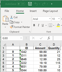
Call the read_excel to read the three files.
final = pd.DataFrame()
for f in glob.glob('C:\\data\*_2*.xlsx'):
   df = pd.read_excel(f, converters={'ID' : str}).set_index("ID")
   final = final.append(df, ignore_index=False, sort=False)

print(final)
      Amount  Quantity
ID
1042   99.89        21
3311   59.99        12
9846   12.99        25
2222   19.19       115
8931   79.99         2
0044  199.89        10
8731   49.99         2
7846  129.00        45
1111   89.19        15
2231   99.99         1
0002   79.89        43
2811   19.99        19
8468  112.99        25
3333  129.99        11
9318   69.99        12
An alternative to retrieving a list of fully qualified file names is retrieving filenames relative to the current working directory executing the session. Import the <a href="https://docs.python.org/3/library/os.html"os module to determine the location for the Python’s current working directory followed by a call to change the working directory to a new location.
import os

wd = os.getcwd()
print (wd)
C:\Users\randy\Desktop\Py_Source
Change working directory.
os.chdir('C:\\data')
wd = os.getcwd()
csv_files = glob.glob('*.csv')
print(csv_files)
['dataframe.csv', 'dataframe2.csv', 'Left.csv', 'messy_input.csv', 'Right.csv', 'Sales_Detail.csv', 'School_Scores.csv', 'scores.csv', 'Tickets.csv']
Illustrate a similar approach for appending and reading multiple .csv files with SAS.
filename tmp pipe 'dir "c:\data\*_2*.csv" /s/b';

data _null_;
   infile tmp;
   length file_name $ 128;
   input file_name $;

   length imported $500;
   retain imported ' ';

   imported = catx(' ',imported,cats('temp',put(_n_,best.)));
   call symput('imported',strip(imported));

      call execute('proc import datafile="'
                    || strip(file_name)
                    || '" out=temp'
                    || strip(put(_n_,best.))
                    || ' dbms=csv replace; run;'
                   );
run;

data final;
   set temp1
       temp2
       temp3;
run;

proc print data=final;
run;

Write .csv
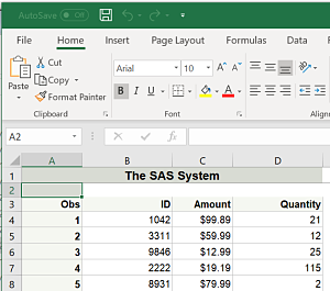
Illustrate the <a href="https://pandas.pydata.org/pandas-docs/stable/reference/api/pandas.DataFrame.to_csv.html"to_csv writer.
final.to_csv('C:\\data\\final.csv', header=True)
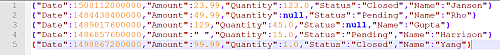
The writer does not return any information to the console to indicate the operation’s success. The image below displays the first 5 rows of the output file, in this case, C:\data\final.csv.

The SAS analog calls PROC EXPORT to write the contents of a SAS dataset to a .csv file.
filename out_csv "c:\data\final_ds.csv";
   proc export data = final
               outfile = out_csv
               dbms = csv;
run;
NOTE: The file OUT_CSV is:
      Filename=c:\data\final_ds.csv,
      RECFM=V,LRECL=32767,File Size (bytes)=0,
      Last Modified=12Nov2018:10:13:47,
      Create Time=12Nov2018:10:13:47

NOTE: 16 records were written to the file OUT_CSV.
      The minimum record length was 11.
      The maximum record length was 18.
NOTE: There were 15 observations read from the data set WORK.FINAL.

15 records created in OUT_CSV from FINAL.

NOTE: "OUT_CSV" file was successfully created.
Write .xls
Write multiple DataFrames to a book of Excel sheets using the to_excel writer. The arguments are largely the same as the to_csv writer.
final.to_excel('C:\\data\\final.xls', merge_cells=False)
There are multiple ways to output a SAS dataset to .xls files. PROC EXPORT provides a convenient approach, but, limits the control over appearances. Alternatively, for finer control over appearances, use ODS tagsets.ExcelXP.
ods tagsets.ExcelXP
   file="c:\data\final_ds.xls"
   style=statistical
   options(frozen_headers='1'
           embedded_titles='yes'
           default_column_width='18');

proc print data=final;
run;

ods tagsets.excelxp close;
run;
If you are using SAS Display Manager to generate this example, you may need to disable the 'View Results as they are generated feature'. This is found by going to the SAS Tools menu in Display Manager option and selecting Options -> Preferences and then selecting the Results tab. Uncheck the box labeled "View results as they are generated".
Read JSON
JSON stands for JavaScript Object Notation and is a well-defined structure for exchanging data among different applications. JSON is designed to to be read by humans and easily parsed by programs. It is relied upon to transmit data through RESTful web services and APIs.
This example creates the jobs DataFrame calling Github’s Jobs API over https using the read_json reader to return posted positions.
Details on the Github jobs API are here.
Print the column labels.
jobs = pd.read_json("https://jobs.github.com/positions.json?description=python")
print(jobs.columns)
Index(['company', 'company_logo', 'company_url', 'created_at', 'description',
       'how_to_apply', 'id', 'location', 'title', 'type', 'url'],
      dtype='object')
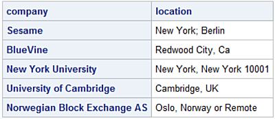
Slice the columns requesting company and location and display the first five rows.
print(jobs[['company', 'location']].head(5))
                       company                  location
0                       Sesame          New York; Berlin
1                     BlueVine          Redwood City, Ca
2          New York University  New York, New York 10001
3      University of Cambridge             Cambridge, UK
4  Norwegian Block Exchange AS    Oslo, Norway or Remote
SAS provides different methods for reading JSON files. The simpliest method is to use the JSON LIBNAME access method.
filename response temp;

proc http
   url="https://jobs.github.com/positions.json?description=python"
   method= "GET"
   out=response;
run;

libname in_json JSON fileref=response;

proc copy in=in_json
          out=work;
run;

proc print data=work.root (obs=5);
   id company;
   var location;
run;
To execute this example the SAS session must be executed with an encoding of UTF-8. By default, SAS sessions executing under Windows use WLATIN1 encoding which can lead to transcoding errors when calling the JSON LIBNAME engine reading UTF-8 formatted records.
Use the following PROC OPTIONS statement to determine the encoding method used by the SAS session.
proc options option=encoding; run;
    SAS (r) Proprietary Software Release 9.4  TS1M5

ENCODING=UTF-8    Specifies the default character-set encoding for the SAS session.
SAS encoding options can only be changed at initialization time. This is controlled by the sasv9.cfg configuration file. The default location on Windows is:
C:\Program Files\SASHome\SASFoundation\9.4\nls\en\sasv9.cfg
Write JSON
Illustrate the to_json writer to write the contents of a DataFrame to a JSON file.
df8.drop(columns = ['Day', 'Month', 'Year'], inplace = True)
df8.to_json("c:\\data\\df8_output.json", orient='records', lines=True)
Illustrate PROC JSON output a SAS Dataset to a JSON file. PROC JSON was introduced with Base SAS Release 9.4.
proc json out='c:\data\sas_final.json' pretty
                                       nosastags;
   export final;
run;
Read RDBMS Table
The pandas.io.sql module provides a set of query wrappers enabling data retrieval while minimizing dependencies on RDBMS-specific APIs. Another way of saying this is, the clever folks who brought you pandas also figured out they can avoid re-inventing wheels by utilizing the SQLAlchemy library as an abstraction to the various databases. This reduces database-dependent code pandas need internally to read and write data using ODBC-compliant engines.
By using the SQLAlchemy library to read RDBMS tables (and queries), you pass SQLAlchemy Expression language constructs which are database-agnostic to the target database. This is analogous to PROC SQL's behavior of using general SAS PROC SQL constructs which are translated for a specific a database without knowing the RDBMS SQL dialect.
See the details configuring, and integrating SQL/Server on Windows with Python here.
Assuming the engine object is defined use the read_sql_table method to read all or subsets of database artifacts such as tables and views. read_sql_table needs two arguments; the target database table, in this case, DimCustomer table and the engine object defining the connection string to the target database.
import pandas as pd
t0 = pd.read_sql_table('DimCustomer', engine)
t0.info()
<class 'pandas.core.frame.DataFrame'>
RangeIndex: 18484 entries, 0 to 18483
Data columns (total 29 columns):
CustomerKey             18484 non-null int64
GeographyKey            18484 non-null int64
CustomerAlternateKey    18484 non-null object
Title                   101 non-null object
FirstName               18484 non-null object
MiddleName              10654 non-null object
LastName                18484 non-null object
NameStyle               18484 non-null bool
BirthDate               18484 non-null datetime64[ns]
MaritalStatus           18484 non-null object
Suffix                  3 non-null object
Gender                  18484 non-null object
EmailAddress            18484 non-null object
YearlyIncome            18484 non-null float64
TotalChildren           18484 non-null int64
NumberChildrenAtHome    18484 non-null int64
EnglishEducation        18484 non-null object
SpanishEducation        18484 non-null object
FrenchEducation         18484 non-null object
EnglishOccupation       18484 non-null object
SpanishOccupation       18484 non-null object
FrenchOccupation        18484 non-null object
HouseOwnerFlag          18484 non-null object
NumberCarsOwned         18484 non-null int64
AddressLine1            18484 non-null object
AddressLine2            312 non-null object
Phone                   18484 non-null object
DateFirstPurchase       18484 non-null datetime64[ns]
CommuteDistance         18484 non-null object
dtypes: bool(1), datetime64[ns](2), float64(1), int64(5), object(20)
memory usage: 4.0+ MB
The BirthDate column is automatically mapped to a datetime64.
If needed, the read_sql_table reader accepts the parse_dates argument to coerce date and datetime columns into a datetime64 type with:
parse_dates={'BirthDate': {'format': '%Y-%m-%d'}}
using nested dictionary key/value pairs where the key is the name of the column followed by another dictionary where its key is 'format' and the value is the desired format directives.
To return a subset of columns from a database table use the columns= argument.
The call to the read_sql_table method contains three arguments. The first argument is the target table DimCustomer; second argument is the engine object containing the connection information for access to the database instance; third is columns= which forms the SELECT list ultimately executed as a T-SQL query on the database instance.
col_names = ['FirstName', 'LastName', 'BirthDate', 'Gender', 'YearlyIncome', 'CustomerKey']
tbl = 'DimCustomer'

t1 = pd.read_sql_table(tbl, engine, columns=col_names)
t1.info()
<class 'pandas.core.frame.DataFrame'>
RangeIndex: 18484 entries, 0 to 18483
Data columns (total 6 columns):
FirstName       18484 non-null object
LastName        18484 non-null object
BirthDate       18484 non-null datetime64[ns]
Gender          18484 non-null object
YearlyIncome    18484 non-null float64
CustomerKey     18484 non-null int64
dtypes: datetime64[ns](1), float64(1), int64(1), object(3)
memory usage: 866.5+ KB
Use the index_col= argument to map input columns as the DataFrame index to create row labels.
t2 = pd.read_sql_table(tbl, engine, columns=col_names, index_col='CustomerKey')
print(t2[['FirstName', 'LastName', 'BirthDate']].head(5))
             FirstName LastName  BirthDate
CustomerKey
11000              Jon     Yang 1971-10-06
11001           Eugene    Huang 1976-05-10
11002            Ruben   Torres 1971-02-09
11003          Christy      Zhu 1973-08-14
11004        Elizabeth  Johnson 1979-08-05
Print the index.
print(t2.index)
Int64Index([11000, 11001, 11002, 11003, 11004, 11005, 11006, 11007, 11008, 11009,
. . .
29474, 29475, 29476, 29477, 29478, 29479, 29480, 29481, 29482,
29483],
dtype='int64', name='CustomerKey', length=18484)
Query RDBMS Table
As part of an analysis effort we often need to execute SQL queries returning rows and columns to construct a DataFrame. Use the read_sql_query reader to send an SQL query to the database and form a DataFrame from the results set.
q1 = pd.read_sql_query('SELECT FirstName, LastName, Gender, BirthDate, YearlyIncome '
                 'FROM dbo.DimCustomer '
                 'WHERE YearlyIncome > 50000; '
                        , engine)
print(q1[['FirstName', 'LastName', 'BirthDate']].tail(5))
     FirstName LastName   BirthDate
9853     Edgar    Perez  1964-05-17
9854     Alvin      Pal  1963-01-11
9855    Wesley    Huang  1971-02-10
9856     Roger    Zheng  1966-03-02
9857    Isaiah  Edwards  1971-03-11
The first argument to the read_sql_query is a valid T-SQL query followed by the engine object holding the connection information to the database to create the q1 DataFrame. Notice how each line of the SQL query uses single quotes and a space (ASCII 32) before the close quote.
The SAS analog uses ODBC Access to SQL Server. This example has the same SELECT list as above. Use PROC PWENCODE to encode password strings so as not to store them as clear-text. Alternatively, you can assign your encoded password string to a SAS macro variable with:
proc pwencode in='YOUR_PASSWORD_HERE' out=pwtemp;
run;
This defines the Macro variable &pwtemp holding the encoded password string.
proc pwencode in=<Your_SQL_Server_PW>;
run;
{SAS002}XXXXXXXXXXXXXXXXXXXXXXXXXXXXA2522
Pass a RDBMS-specific query to SQL/Server using a pass-thru query.
libname sqlsrvr odbc
        uid=randy
        pwd={SAS002}XXXXXXXXXXXXXXXXXXXXXXXXXXXXA2522
        datasrc=AdventureWorksDW
        bulkload=yes;

title1 "Default Informats and Formats";
proc sql;
   create table customers as
   select FirstName
         ,LastName
         ,BirthDate
         ,Gender
         ,YearlyIncome
         ,CustomerKey
   from sqlsrvr.DimCustomer;

   select name
         ,informat
         ,format
    from DICTIONARY.COLUMNS
    where libname = 'WORK' &
          memname = 'CUSTOMERS';
quit;
The second PROC SQL SELECT statements queries the DICTIONARY.COLUMNS table to return formats and informats assigments to the WORK.CUSTOMERS columns. SAS formats and informats are analogous to column types, in that the informat directs how values are read on input and formats direct how values are written on output.
In this case the incoming SQL Server table values for the BirthDate column are read using the SAS $10. informat treating the values as a 10-byte long character string.

To utilize the BirthDate variable with SAS datetime expressions a subsequent Data Step is needed to copy the these variable values into a numeric variable to allow datetime handling.
Unlike Python, existing SAS variables can not be recast. In order to output the customers dataset with the BirthDate variable with a datetime format requires copying the dataset, renaming the BirthDate variable to dob and assigning its values to the output BirthDate variable calling the INPUT function.
Illustrates copying the customers dataset and using the INPUT function to load the original character values from the BirthDate variable to a numeric variable and assign it a permanent format of yymmdd10..
data customers(drop = dob);
   set customers(rename=(BirthDate = dob));
   length BirthDate 8;

BirthDate = input(dob,yymmdd10.);
format BirthDate yymmdd10.;
run;

 title1 "Modified Informats and Formats";
proc sql;
   select name
         ,informat
         ,format
   from DICTIONARY.COLUMNS
      where libname = 'WORK' &
           memname = 'CUSTOMERS';
quit;
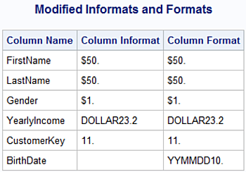
Not all SQL queries return a results set. Illustrates using the sql.execute statement. This is useful for queries not returning results sets such as CREATE TABLE, DROP, or INSERT statements, etc. These SQL statements are specific to the target RDBMS.
Connect to the database.
from pandas.io import sql
sql.execute('USE AdventureWorksDW2017; ', engine)
<sqlalchemy.engine.result.ResultProxy object at 0x0000020172E0DE80>
DROP the CustomerPy (if it already exists then the CREATE TABLE will fail) followed by the CREATE TABLE statement.
sql.execute('DROP TABLE CustomerPy', engine)

sql.execute("CREATE TABLE CustomerPy (ID int,           \
...             Name nvarchar(255),                         \
...             StartDate date);", engine)
<sqlalchemy.engine.result.ResultProxy object at 0x0000020172E0D898>
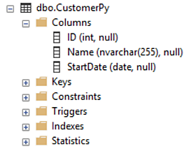
Displays column attributes for the created SQL Server table CustomerPy.
Illustrate SQL pass-thru as a wrapper to pass T-SQL statements directly to SQL/Server through the ODBC API. This example is the analog to the above sql.execute statements passing SQL to the database which do not return a results set.
proc sql;
connect to odbc as sqlsrvr
(dsn=AdventureWorksDW
uid=randy
password=
{SAS002}XXXXXXXXXXXXXXXXXXXXXXXXXXXXA2522);
exec
(CREATE TABLE CustomerPy (ID int,
Name nvarchar(255),
StartDate date)) by sqlsrvr;
%put Note: Return Code for SQL Server is: &sqlxrc;
%put Note: Return Message for SQL Server is: &sqlxmsg;
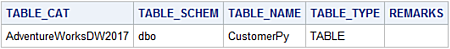
select * from connection to sqlsrvr
(ODBC::SQLTables (,,"CustomerPy",));
disconnect from sqlsrvr;
%put Note: Return Code for SQL Server is: &sqlxrc;
%put Note: Return Message for SQL Server is: &sqlxmsg;
quit;
With SAS SQL Pass-Thru any statements inside a parenthesized expression are passed directly to the database library API, in this case, ODBC.
CREATE TABLE CustomerPy (ID int,
                    Name nvarchar(255),
                    StartDate date)
SAS/Access to ODBC supports calls to the ODBC::SQLAPI. This interface is an alternative to querying the RDBMS catalog tables. In this example:
(ODBC::SQLTables (,,"CustomerPy",));
returns information about the created CustomerPy SQL/Server table.
Write RDBMS Table
The pandas library provisions the ability to write DataFrames as RDBMS tables with the to_sql writer.
Generate the df_dates DataFrame as a source to write to a SQL/Server table.
date_rng = pd.date_range(start='1/1/2019', end='1/31/2019', freq='D')
df_dates = pd.DataFrame(date_rng, columns=['dates'])
df_dates['rnd_values'] = np.random.randint(100,999,size=(len(date_rng)))
print(df_dates.head(5))
       dates  rnd_values
0 2019-01-01         792
1 2019-01-02         102
2 2019-01-03         534
3 2019-01-04         187
4 2019-01-05         240
Illustrate the df_dates DataFrame calling the to_sql method attempting to create the SQLTableFromDF SQL Server table.
df_dates.to_sql('SQLTableFromDF', engine, if_exists='replace', index=False)
In cases where a large DataFrame is written as an RDBMS table the call may return an ODBC error like:
pyodbc.ProgrammingError: ('42000', '[42000] [Microsoft][ODBC SQL Server Driver][SQL Server]The incoming request has too many parameters. The server supports a maximum of 2100 parameters. Reduce the number of parameters and resend the request. (8003)
then use the chunksize= argument.
df_dates.to_sql('SQLTableFromDF', engine, if_exists='replace', chunksize=100, index=False)
Unlike SAS , when the to_sql method writes to the table it does not return messages or provide a return code. So send a query to SQL/Server's catalog table information_schema.columns to validate its existence.
confirm1 = pd.read_sql_query("SELECT column_name as 'COL_NAME', "
           "data_type as 'Data_Type', "
           "IS_NULLABLE as 'Nulls Valid' "
           "FROM information_schema.columns "
           "WHERE table_name = 'SQLTableFromDF' ", engine)
print(confirm1)
     COL_NAME Data_Type Nulls Valid
0       dates  datetime         YES
1  rnd_values       int         YES
Each physical line in the call to read_sql_query reader requires double quotes. Single quotes label column headings following the T-SQL AS keyword along with single quotes used in the WHERE clause. Single quotes are passed since they are a required for a valid T-SQL query.
Write RDBMS NULLS
Missing values between data formats can be challenging at times since each data format uses different sentinel values to indicate 'missing' or NULL's.
In the case of a DataFrame, missing values can be NaN for float64s and NaT (for Not a Time) for datetime64 types. Insert missing values into the df_dates DataFrame to ensure subsequent SQL queries properly handle the missing values.
import numpy as np
df_dates.loc[df_dates['rnd_values'] > 200, 'rnd_values'] = np.NaN
df_dates.loc[df_dates['rnd_values'] > 100, 'dates'] = np.NaN
df_dates.isnull().sum()
dates         2
rnd_values    5
dtype: int64
Print the first 4 rows.
print(df_dates.head(4))
       dates  rnd_values
0 2019-01-01         NaN
1 2019-01-02         NaN
2 2019-01-03         NaN
3        NaT       169.0
Write the df_dates DataFrame as the SQLTableFromDF2 SQL/Server table and then read the rows into the confirm2 DataFrame and print them.
df_dates.to_sql('SQLTableFromDF2', engine, if_exists='replace', chunksize=100, index=False)
confirm2 = pd.read_sql_query("SELECT TOP 5 * "
                             "FROM SQLTableFromDF2 "
                              "WHERE rnd_values is NULL or dates is NULL ", engine)

print(confirm2)
       dates  rnd_values
0 2019-01-01         NaN
1 2019-01-02         NaN
2 2019-01-03         NaN
3        NaT       169.0
4 2019-01-05         NaN
Calling the print function for the confirm2 DataFrame displays the values for the dates and rnd_values columns made the round-trip from DataFrame to SQL Server and back maintaining the integrity of missing values between both formats.
Read SAS Datasets
pandas provide the read_sas reader to create DataFrames from permanent SAS datsets. Permanent SAS datasets are often refered to as .sas7bdat files (after the extension SAS uses to name dataset files on Windows and Unix filesystems).
Generate the to_df permanent SAS Dataset written to C:\data`` recongized by Windows as the file:C:\data\to_df.sas7bdat```.
libname out_data 'c:\data';

data out_data.to_df;
   length even_odd $ 4;
   call streaminit(987650);
   do datetime = '01Dec2018 00:00'dt to '02Dec2018 00:00'dt by 60;
      amount = rand("Uniform", 50, 1200);
      quantity = int(rand("Uniform", 1000, 5000));

       if int(mod(quantity,2)) = 0 then even_odd = 'Even';
            else even_odd = 'Odd';
       output;
   end;
format datetime datetime16.
       amount dollar12.2
       quantity comma10.;
run;
Illustrate the read_sas method.
from_sas = pd.read_sas("c:\\Data\\to_df.sas7bdat",
                        format='SAS7BDAT',
                        encoding = 'latin-1')
from_sas.info()
<class 'pandas.core.frame.DataFrame'>
RangeIndex: 1441 entries, 0 to 1440
Data columns (total 4 columns):
even_odd    1441 non-null object
datetime    1441 non-null datetime64[ns]
amount      1441 non-null float64
quantity    1441 non-null float64
dtypes: datetime64[ns](1), float64(2), object(1)
memory usage: 45.1+ KB
Print the first 5 rows of the from_sas DataFrame.
print(from_sas.head(5))
  even_odd            datetime       amount  quantity
0      Odd 2018-12-01 00:00:00   340.629296    3955.0
1     Even 2018-12-01 00:01:00  1143.526378    1036.0
2     Even 2018-12-01 00:02:00   209.394104    2846.0
3     Even 2018-12-01 00:03:00   348.086155    1930.0
4     Even 2018-12-01 00:04:00   805.929860    3076.0
The call to the read_sas reader has as the first argument the Windows’s pathname to the OUT_DATA.TO_DF dataset (as it is known to SAS). The second argument, format= is SAS7BDAT. If the SAS dateset is in transport format then this value is XPORT. The third argument, encoding= is set to latin-1 to match the encoding for the to_df.sas7bdat dataset.
The read_sas reader issues a file lock for the target input in for reading. This can cause file contention issues if you attempt to open the SAS dataset for output while calling the read_sas reader. The SAS log issues the error:
ERROR: A lock is not available for OUT_DATA.TO_DF.DATA.
NOTE: The SAS System stopped processing this step because of errors.
WARNING: The data set OUT_DATA.TO_DF was only partially opened and will not be saved.
If encountered ending the Python session calling the read_sas reader releases the lock.
The pandas I/O library does not provide a write_sas method. Using SAS Institute’s open-source SASPy module enables bi-directional interchange between panda DataFrames and SAS datasets.