Introduction
pandas have two main facilities for combining DataFrames with various types of set logic and relational/algebraic capabilities for join/merge operations. The concat method performs row-wise or column-wise concatenation operations and performs union and intersection set logic on DataFrames.
pandas merge method offers a SQL-like interface for performing DataFrame join/merge operations. The SAS MERGE statement and PROC SQL are the analogs used to introduce the merge method.
Construct the left and right DataFrames with the ID column as a common key.
import pandas as pd
url_l = "https://raw.githubusercontent.com/RandyBetancourt/PythonForSASUsers/master/data/Left.csv"
left = pd.read_csv(url_l)
url_r = "https://raw.githubusercontent.com/RandyBetancourt/PythonForSASUsers/master/data/Right.csv"
right = pd.read_csv(url_r)
Display the left DataFrame.
print(left)
    ID       Name Gender   Dept
0  929     Gunter      M    Mfg
1  446  Harbinger      M    Mfg
2  228     Benito      F    Mfg
3  299   Rudelich      M  Sales
4  442  Sirignano      F  Admin
5  321   Morrison      M  Sales
6  321   Morrison      M  Sales
7  882     Onieda      F  Admin
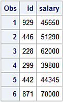
Display the Right DataFrame.
print(right)
    ID  Salary
0  929  45,650
1  446  51,290
2  228  62,000
3  299  39,800
4  442  44,345
5  871  70,000
The left DataFrame has has the duplicate value 321 for the ID column making a many-to-one relationship between these DataFrames. The right DataFrame has an ID value of 871 not found in the left DataFrame. These are the types of issues often causing unexpected results when performing merge/join operations.
Build the left and right SAS datasets.
data left;
infile datalines dlm=',';
length name $ 12
dept $ 5;
input name $
id
gender $
dept;
list;
datalines;
Gunter, 929, M, Mfg
Harbinger, 446, M, Mfg
Benito, 228, F, Mfg
Rudelich, 299, M, Sales
Sirignano, 442, F, Admin
Morrison, 321, M, Sales
Morrison, 321, M, Sales
Oniedae, 882, F, Admin
;;;;
data right;
input id
salary;
list;
datalines;
929 45650
446 51290
228 62000
299 39800
442 44345
871 70000
;;;;
run;
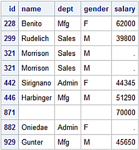
proc print data=left;
run;
proc print data=right;
run;
left Dataset
 right Dataset
SAS Sort/Merge
SAS Sort/Merge, also referred to as match-merge is a common pattern for match-merging two SAS datasets with a common key. The left and right SAS datasets are sorted by the id variable enabling BY-Group processing. After sorting, the match merge operation joins the datasets by their common id variable.
Experienced SQL users know the results from this match-merge are the same as an outer join in PROC SQL in cases where table relationships are one-to-one or many-to-one. In cases where the table relationships are many-to-many, results from the Data Step and PROC SQL differ. At the end of this section are the many-to-many join use cases for SAS and pandas.
Perform a SAS Sort/Merge to combine observations from the left and right datasets into a single observation in the merge_lr dataset according to the values for the id variable in the datasets.
proc sort data=left;
by id;
run;
proc sort data=right;
by id;
run;
data merge_lr;
merge left
right;
by id;
run;
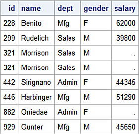
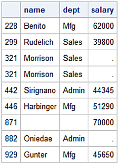
proc print data=merge_lr;
id id;
run;
merge_lr dataset
Introduce pandas merge method using a single Data Step to create seven output datasets to illustrate the following operations:
1. Inner Join
2. Right Join
3. Left Join
4. Outer Join
5. Right Join Unmatched Keys
6. Left Join Unmatched Keys
7. Outer Join Unmatched Keys
data inner
     right
     left
     outer
     nomatch_l
     nomatch_r
     nomatch;

merge left(in=l)
      right(in=r);
by id;

if (l=l and r=1) then output inner; *Inner Join;

if r = 1 then output right; * Right Join;

if l = 1 then output left;  * Left Join;

if (l=1 or r=1) then output outer; *Outer Join;

if (l=1 and r=0) then output nomatch_l;

if (l=0 and r=1) then output nomatch_r;

if (l=0 or r=0) then output nomatch;

run;
NOTE: There were 8 observations read from the data set WORK.LEFT.
NOTE: There were 6 observations read from the data set WORK.RIGHT.
NOTE: The data set WORK.INNER has 6 observations and 5 variables.
NOTE: The data set WORK.RIGHT has 6 observations and 5 variables.
NOTE: The data set WORK.LEFT has 8 observations and 5 variables.
NOTE: The data set WORK.OUTER has 9 observations and 5 variables.
NOTE: The data set WORK.NOMATCH_L has 3 observations and 5 variables.
NOTE: The data set WORK.NOMATCH_R has 1 observations and 5 variables.
NOTE: The data set WORK.NOMATCH has 4 observations and 5 variables.
Inner Join
SAS Data Step inner join returns matching rows.
data inner;
   merge left(in=l)
         right(in=r);
by id;

if (l=1 and r=1) then output;
run;
NOTE: There were 8 observations read from the data set WORK.LEFT.
NOTE: There were 6 observations read from the data set WORK.RIGHT.
NOTE: The data set WORK.INNER has 5 observations and 5 variables.
The SAS dataset IN= option create a Boolean variable indicating which dataset contributes values from the current observation being read.
The pandas merge method signature:
pd.merge(left, right, how='inner', on=None, left_on=None,
         right_on=None, left_index=False, right_index=False,
         sort=False, suffixes=('_x', '_y'), copy=True,
         indicator=False, validate=None)
pandas inner join uses the on='ID' argument indicating the ID column is a key column found in both DataFrames. The on='ID' argument is not needed in the example below, since the merge method detects the presence of the ID column in both DataFrames and automatically asserts them as key columns. The how='inner' argument performs an inner join, which is the default.
inner = pd.merge(left, right, on='ID', how='inner', sort=False)
print(inner)
    ID       Name Gender   Dept  Salary
0  929     Gunter      M    Mfg  45,650
1  446  Harbinger      M    Mfg  51,290
2  228     Benito      F    Mfg  62,000
3  299   Rudelich      M  Sales  39,800
4  442  Sirignano      F  Admin  44,345
PROC SQL query for an inner join.
proc sql;
   select *
from left
    ,right
where left.id = right.id;
quit;
An alternative syntax uses the PROC SQL keywords INNER JOIN. The join predicate l.id = r.id must be true row rows be included in the results set.
proc sql;
select *
   from left as l
inner join
   right as r
on l.id = r.id;
quit;
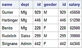
Inner join results
Right Join
A right join returns all observations from the right dataset along with any observations from the left dataset where the id variable values match in both datasets. In cases where there are observations in the right dataset with no matching id values in the left dataset these values are set to missing.
data r_join;
   merge left(in=l)
         right(in=r);
   by id;

if r=1 then output;
run;
NOTE: There were 8 observations read from the data set WORK.LEFT.
NOTE: There were 6 observations read from the data set WORK.RIGHT.
NOTE: The data set WORK.R_JOIN has 6 observations and 5 variables.
Call the merge method using the how='right' argument to perform a right join. The merge method automatically coalesces the ID column values from both DataFrames into a single column in the returned r_join DataFrame. In cases where there are rows in the right DataFrame with no matching ID values in the left DataFrame these values are set to NaN's.
r_join = pd.merge(left, right, how='right', sort=True)
print(r_join)
    ID       Name Gender   Dept  Salary
0  228     Benito      F    Mfg  62,000
1  299   Rudelich      M  Sales  39,800
2  442  Sirignano      F  Admin  44,345
3  446  Harbinger      M    Mfg  51,290
4  871        NaN    NaN    NaN  70,000
5  929     Gunter      M    Mfg  45,650
Call PROC SQL query for a right join. The COALESCE function coerces the id columns from both tables to return a single column. Without the COALESCE function the results set returns the id column from both tables with the id values from the left table set to null for rows with no matching values found for the id column from the right table.
proc sql;
   select coalesce(left.id, right.id) as id
         ,name
         ,dept
         ,gender
         ,salary
   from left
   right join
      right
   on left.id = right.id;
quit;
Display right join results set.

Left Join
A left join returns all rows from the left table along with any rows from the right table where the join predicate is true. In this case, all rows from the left dataset are returned along with any rows in the right dataset with id values matching in the left dataset.
data l_join;
merge left(in=l)
       right(in=r);
by id;

if l=1 then output;
run;
NOTE: There were 8 observations read from the data set WORK.LEFT.
NOTE: There were 6 observations read from the data set WORK.RIGHT.
NOTE: The data set WORK.L_JOIN has 8 observations and 5 variables.
Call the merge method using the how='left' arugment to perform a left join. It automatically coalesces the ID column values from both DataFrames into a single column in the returned l_join DataFrame. The output shows all rows from the left DataFrame returned with NaN’s for columns in the right DataFrame having unmatched values from the ID column in the left DataFrame.
l_join = pd.merge(left, right, how='left', sort=False)
print(l_join)
    ID       Name Gender   Dept  Salary
0  929     Gunter      M    Mfg  45,650
1  446  Harbinger      M    Mfg  51,290
2  228     Benito      F    Mfg  62,000
3  299   Rudelich      M  Sales  39,800
4  442  Sirignano      F  Admin  44,345
5  321   Morrison      M  Sales     NaN
6  321   Morrison      M  Sales     NaN
7  882     Onieda      F  Admin     NaN
PROC SQL query for an left join.
proc sql;
   select coalesce(left.id, right.id) as id
         ,name
         ,dept
         ,gender
         ,salary
   from left
      left join
           right
on left.id = right.id;
quit;
Like the above SAS right join, this example uses the COALESCE function to coerce the id columns from both tables to return a single column.
Left join results
Outer Join
The SAS Sort/Merge returns the same results set as those from PROC SQL outer joins in cases where the table relationships are either one-to-one or one-to-many. The results from this example are the same as the SAS Sort/Merge results above.
Perform an outer join with the how='outer' argument to select all rows from the left and right DataFrames. In cases where there are no matched values for the ID column these values are set to NaN's.
merge_lr = pd.merge(left, right, on='ID', how='outer', sort=True)
print(merge_lr)
    ID       Name Gender   Dept  Salary
0  228     Benito      F    Mfg  62,000
1  299   Rudelich      M  Sales  39,800
2  321   Morrison      M  Sales     NaN
3  321   Morrison      M  Sales     NaN
4  442  Sirignano      F  Admin  44,345
5  446  Harbinger      M    Mfg  51,290
6  871        NaN    NaN    NaN  70,000
7  882     Onieda      F  Admin     NaN
8  929     Gunter      M    Mfg  45,650
PROC SQL Outer Join.
proc sql;
   select coalesce(left.id, right.id)
         ,name
         ,dept
         ,salary
    from left
full join
     right
on left.id = right.id;
quit;
All rows from the left and right tables are returned. In cases where there are no matched values for the id column values are set to missing.
Outer join results
Right Join Unmatched Keys
The examples above are based on finding matched key values in the data to be joined. The next three examples illustrate joining data where keys are unmatched.
Every SQL join is either a Cartesian product join or a sub-set of a Cartesian product join. With unmatched key values a form of WHERE filtering is needed.
The SAS Data Step with its IN= Dataset option and associated IF logic is a common pattern for this filtering. PROC SQL with a WHERE clause is also used.
The next three pandas examples illustrate the indicator= argument for the merge method as an analog to the SAS IN= dataset option. For pandas the filtering process utilizes a Boolean comparison based on this indicator= value.
Data Step Unmatched Keys in Right.
data r_join_nmk;
   merge left(in=l)
         right(in=r);
by id;

if (l=0 and r=1) then output;
run;
NOTE: There were 8 observations read from the data set WORK.LEFT.
NOTE: There were 6 observations read from the data set WORK.RIGHT.
NOTE: The data set WORK.R_JOIN_NMK has 1 observations and 5 variables.
Right join on unmatched keys in DataFrames with the indicator= argument. This argument adds a column to the output DataFrame with the default name _merge as an indicator for the source of each row. Returned values are:
- left_only
- right_only
- both
By applying a Boolean filter to the indicator= values, we replicate the behavior of the SAS IN= Dataset option.
pandas right join with unmatched keys. Override the indicator= argument to label the new column in_col and display results before filtering.
nomatch_r = pd.merge(left, right, on='ID', how='outer', sort=False, indicator='in_col')
print('\n',
      nomatch_r,
      '\n')
     ID       Name Gender   Dept  Salary      in_col
0  929     Gunter      M    Mfg  45,650        both
1  446  Harbinger      M    Mfg  51,290        both
2  228     Benito      F    Mfg  62,000        both
3  299   Rudelich      M  Sales  39,800        both
4  442  Sirignano      F  Admin  44,345        both
5  321   Morrison      M  Sales     NaN   left_only
6  321   Morrison      M  Sales     NaN   left_only
7  882     Onieda      F  Admin     NaN   left_only
8  871        NaN    NaN    NaN  70,000  right_only
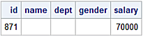
Apply the Boolean operator in order to get the results.
nomatch_r[(nomatch_r['in_col'] == 'right_only')]
    ID Name Gender Dept  Salary      in_col
8  871  NaN    NaN  NaN  70,000  right_only
PROC SQLRight join unmatched keys is generated by adding a WHERE clause to the example from PROC SQL Right Join above.
proc sql;
   select coalesce(left.id, right.id) as id
         ,name
         ,dept
         ,gender
         ,salary

   from left
        right join right on left.ID = right.ID
   where left.ID is NULL;
quit;
Right join unmatched keys results
Left Join Unmatched Keys
SAS Data Step to find the unmatched key values in the left table.
data l_join_nmk;
   merge left(in=l)
         right(in=r);
by id;

if (l=1 and r=0) then output;
run;
NOTE: There were 8 observations read from the data set WORK.LEFT.
NOTE: There were 6 observations read from the data set WORK.RIGHT.
NOTE: The data set WORK.L_JOIN_NMK has 3 observations and 5 variables.
pandas left join unmatched keys. Column values returned from the right DataFrame are set to NaN's.
nomatch_l = pd.merge(left, right, on='ID', how='outer', sort=False, indicator='in_col')
nomatch_l = nomatch_l[(nomatch_l['in_col'] == 'left_only')]

print('\n',
       nomatch_l,
      '\n')
     ID      Name Gender   Dept Salary     in_col
5  321  Morrison      M  Sales    NaN  left_only
6  321  Morrison      M  Sales    NaN  left_only
7  882    Onieda      F  Admin    NaN  left_only
PROC SQL Left Join on Unmatched Keys. The WHERE clause returns rows from the left table having no matching id values in the right table. Column values returned from the right table are set to missing.
proc sql;
   select coalesce(left.id, right.id) as id
         ,name
         ,dept
         ,gender
         ,salary
   from left
   left join
        right
   on left.id = right.id
   where right.id is null;
quit;
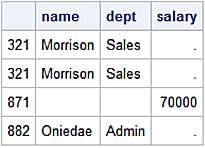
Left join unmatched keys results

Outer Join Unmatched Keys
An outer join on unmatched keys returns rows from each DataFrame with unmatched keys in the other DataFrame.
Find the unmatched key values in the left or right tables.
data outer_nomatch_both;
   merge left (in=l)
   right (in=r);
by id;

if (l=0 or r=0) then output;
run;
NOTE: There were 8 observations read from the data set WORK.LEFT.
NOTE: There were 6 observations read from the data set WORK.RIGHT.
NOTE: The data set WORK.OUTER_NOMATCH_BOTH has 4 observations and 5 variables.
Finding unmatched keys in both DataFrames requires an outer join with a corresponding filter identifying missing values.
Perform pandas outer join on unmatched keys in both DataFrames and display the results before applying a filter.
nomatch_both = pd.merge(left, right, on='ID', how='outer', sort=False, indicator='in_col')

print('\n',
      nomatch_both,
      '\n')
     ID       Name Gender   Dept  Salary      in_col
0  929     Gunter      M    Mfg  45,650        both
1  446  Harbinger      M    Mfg  51,290        both
2  228     Benito      F    Mfg  62,000        both
3  299   Rudelich      M  Sales  39,800        both
4  442  Sirignano      F  Admin  44,345        both
5  321   Morrison      M  Sales     NaN   left_only
6  321   Morrison      M  Sales     NaN   left_only
7  882     Onieda      F  Admin     NaN   left_only
8  871        NaN    NaN    NaN  70,000  right_only
Filter with the Boolean or (|) logic selecting rows where the in_col column value is 'left_only' or where the in_col column value is 'right_only'.
nomatch_both[(nomatch_both['in_col'] == 'right_only') |
(nomatch_both['in_col'] == 'left_only')]
    ID      Name Gender   Dept  Salary      in_col
5  321  Morrison      M  Sales     NaN   left_only
6  321  Morrison      M  Sales     NaN   left_only
7  882    Onieda      F  Admin     NaN   left_only
8  871       NaN    NaN    NaN  70,000  right_only
An alternative Boolean expression that is more Pythonic is:
nomatch_both = nomatch_both[nomatch_both["in_col"] != 'both']
selecting those rows where the in_col column value is not 'both'.
PROC SQL outer join unmatched keys in both datasets.
proc sql;
   select coalesce(left.id, right.id)
         ,name
         ,dept
         ,salary
   from left
   full join
   right
      on left.id=right.id
   where left.id ne right.id;
quit;
The WHERE clause returns rows from the left table having no matching id values in the right table and rows from the right table having no matching id values in the left table.
Outer join unmatched keys results
Joining on an Index
Recall how DataFrame indexes are used as row labels. The pandas library implements the join method to combine columns from two differently-indexed DataFrames into a single DataFrame. The join method is a convenience for calling the merge method in those cases where a DataFrame lacks an index (other than the default RangeIndex) or key columns have different names.
Construct the left and right DataFrames using an index to label rows.
import pandas as pd
left = pd.DataFrame(
    { 'Style' : ['S1', 'S2', 'S3', 'S4'],
      'Size' : ['SM', 'MD', 'LG', 'XL']},
    index = ['01', '02', '03', '05'])

right = pd.DataFrame(
    { 'Color' : ['Red', 'Blue', 'Cyan', 'Pink'],
      'Brand' : ['X', 'Y', 'Z', 'J']},
    index = ['01', '02', '03', '04'])
Display the left DataFrame.
print(left)
   Style Size
01    S1   SM
02    S2   MD
03    S3   LG
05    S4   XL
Display the right DataFrame.
print(right)
  Color Brand
01   Red     X
02  Blue     Y
03  Cyan     Z
04  Pink     J
Call the join method with the default left join using the how='left' argument.
df1 = left.join(right, how='left')

print(df1)
   Style Size Color Brand
01    S1   SM   Red     X
02    S2   MD  Blue     Y
03    S3   LG  Cyan     Z
05    S4   XL   NaN   NaN
The unlabeled indexes from both columns are preserved on the new df1 DataFrame as a function of the type of join called. The row labeled 04 from the right DataFrame is excluded since this is a left join.
The corresponding merge syntax needed to produce the same results is:
df1 = left.merge(right, how='left', left_index=True, right_index=True)
The join method provisions four joining methods as a value to the how= argument.
- Left: Uses the calling DataFrame’s index, or a key column, if specified. This is the default join method.
- Right: Uses the other DataFrame’s index.
- Outer: Returns union of calling DataFrame’s index with the other DataFrame index and sorts the index.
- Inner: Returns intersection of calling DataFrame’s index with the other DataFrame index, preserves the order of the calling DataFrame index.
Outer join on the indexed DataFrames. The how='outer' argument enables an outer join.
df2 = left.join(right, how='outer')
print(df2)
   Style Size Color Brand
01    S1   SM   Red     X
02    S2   MD   Blue    Y
03    S3   LG   Cyan    Z
04   NaN  NaN   Pink    J
05    S4    XL   NaN  NaN
Inner join on Indexed DataFrames.
df3 = left.join(right, how='inner')
print(df3)
   Style Size Color Brand
01    S1   SM   Red     X
02    S2   MD  Blue     Y
03    S3   LG   Cyan    Z
Join Key Column with an Index
In cases where a DataFrame is not indexed use the on= argument to identify the key column used in a join operation.
Construct and display the left DataFrame which has no index.
left = pd.DataFrame(
    {'Style' : ['S1', 'S2', 'S3', 'S4'],
     'Size'  : ['SM', 'MD', 'LG', 'XL'],
     'Key'   : ['01', '02', '03', '05']})

print(left)
  Style Size Key
0    S1   SM  01
1    S2   MD  02
2    S3   LG  03
3    S4   XL  05
Construct and display the right DataFrame with an index.
right = pd.DataFrame(
    {'Color' : ['Red', 'Blue', 'Cyan', 'Pink'],
     'Brand' : ['X', 'Y', 'Z', 'J']},
      index = ['01', '02', '03', '04'])

print(right)
  Color Brand
01   Red     X
02  Blue     Y
03  Cyan     Z
04  Pink     J
Construct the df4 DataFrame calling the join method to perform a left join with the Key column in the left DataFrame as its key and the index in the right DataFrame as its key.
df4 = left.join(right, on='Key', how='outer')
print(df4)
  Style Size Key Color Brand
0    S1   SM  01   Red     X
1    S2   MD  02  Blue     Y
2    S3   LG  03  Cyan     Z
3    S4   XL  05   NaN   NaN
3   NaN  NaN  04  Pink     J
Call the merge method to produce the same results as the above join example.
The how='outer' argument calls for an outer join using the left_on='Key' argument to designate the Key column as the join key for the left Dataframe. The right_index=True argument designates the index as the join key for the right DataFrame.
df5 = pd.merge(left, right, left_on='Key', how='outer', right_index=True)
print(df5)
  Style Size Key Color Brand
0    S1   SM  01   Red     X
1    S2   MD  02  Blue     Y
2    S3   LG  03  Cyan     Z
3    S4   XL  05   NaN   NaN
3   NaN  NaN  04  Pink     J
SAS Many-to-Many Join Use Case
Illustrate differences between results created by the default SORT/MERGE operation and a PROC SQL outer join in those cases where the table relationship is many-to-many. Observe the note in the log:
NOTE: MERGE statement has more than one data set with repeats of BY values.
Many-to_Many relationship with SAS Sort/Merge. Build the left and right datasets and display them.
data left;
   infile datalines dlm=',';
   length color $ 6;
input style
      color;
list;
datalines;
1, Blue
1, Green
2, Blue
2, Green
2, Orange
3, Blue
3, Green
;;;;
run;

data right;
   infile datalines dlm=',';
   length size $ 8;
input style
      size $;
list;
datalines;
1, Small
1, Large
2, Tiny
2, Small
2, Large
2, X-Large
5, Small
;;;;
run;

proc sort data=left;
   by style;
run;

proc sort data=right;
   by style;
run;

data merge_lr;
   merge left
         right;
by style;
run;

proc print data=merge_lr;
   id style;
run;
Call PROC SQL to perform a full outer join on the left and right datasets.
proc sql;
   select coalesce(left.style, right.style)
         ,color
         ,size
   from left
   full join
        right
   on left.style=right.style;
quit;

pandas Many-to-Many Join Use Case
Many-to_Many relationship with pandas merge Sort/Merge. Construct and Dsiplay the left DataFrame.
import pandas as pd
left = pd.DataFrame([[1, 'Blue'],
                     [1, 'Green'],
                     [2, 'Blue'],
                     [2, 'Green'],
                     [2, 'Orange'],
                     [3, 'Blue'],
                     [3, 'Green']],
        columns=['Style', 'Color'])

print(left)
   Style   Color
0      1    Blue
1      1   Green
2      2    Blue
3      2   Green
4      2  Orange
5      3    Blue
6      3   Green
Construct and display the right DataFrame.
right = pd.DataFrame([[1, 'Small'],
                      [1, 'Large'],
                      [2, 'Tiny'],
                      [2, 'Small'],
                      [2, 'Large'],
                      [2, 'X-Large'],
                      [5, 'Small']],
        columns=['Style', 'Size'])
print(right)
   Style     Size
0      1    Small
1      1    Large
2      2     Tiny
3      2    Small
4      2    Large
5      2  X-Large
6      5    Small
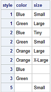
Call the pandas merge method with the how='outer' argument.
outer = pd.merge(left, right, how='outer', sort=False)
print(outer)
    Style   Color     Size
0       1    Blue    Small
1       1    Blue    Large
2       1   Green    Small
3       1   Green    Large
4       2    Blue     Tiny
5       2    Blue    Small
6       2    Blue    Large
7       2    Blue  X-Large
8       2   Green     Tiny
9       2   Green    Small
10      2   Green    Large
11      2   Green  X-Large
12      2  Orange     Tiny
13      2  Orange    Small
14      2  Orange    Large
15      2  Orange  X-Large
16      3    Blue      NaN
17      3   Green      NaN
18      5     NaN    Small