GroupBy Object
A pattern common to data analysis is BY-group processing. It is defined as:
• Splitting vales into groups based on some criteria
• Applying a function to the groups
• Combining the results into a data structure
Creating a DataFrame often with a single pass of the data.
The signature for defining a GroupBy object:
DataFrame.groupby(by=None, axis=0, level=None, as_index=True,
sort=True, group_keys=True, squeeze=False, observed=False,
**kwargs)
Create the df DataFrame and GroupBy object for the District column. A DataFrame GroupBy object is returned rather than a DataFrame. The gb object is analagous to a SQL view containing instructions to execute SQL statement to materialize rows and columns when the view is applied.
import pandas as pd
df = pd.DataFrame(
    [['I',  'North', 'Patton',   17,  27,  22],
    ['I',   'South', 'Joyner',   13,  22,  19],
    ['I',   'East',  'Williams', 111, 121, 29],
    ['I',   'West',  'Jurat',    51,  55,  22],
    ['II',  'North', 'Aden',     71,  70,  17],
    ['II',  'South', 'Tanner',   113, 122, 32],
    ['II',  'East',  'Jenkins',  99,  99,  24],
    ['II',  'West',  'Milner',   15,  65,  22],
    ['III', 'North', 'Chang',    69,  101, 21],
    ['III', 'South', 'Gupta',    11,  22,  21],
    ['III', 'East',  'Haskins',  45,  41,  19],
    ['III', 'West',  'LeMay',    35,  69,  20],
    ['III', 'West',  'LeMay',    35,  69,  20]],
    columns=['District', 'Sector', 'Name', 'Before', 'After', 'Age'])

gb = df.groupby(['District'])
print(gb)
<pandas.core.groupby.generic.DataFrameGroupBy object at 0x000002592A6A3B38>
An approximate SQL analogy.
CREATE VIEW GB as
   SELECT distinct District
                 , sum(Before)
                 , sum(After)
   FROM DF
   GROUP BY District
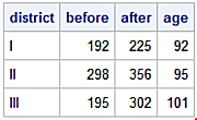
When the GroupBy object is applied results are produced. Create the d_grby_sum DataFrame by adding the numeric columns for each District. All numeric columns in the df Dataframe are grouped by the unique levels of the District column and summed within the group.
d_grby_sum = df.groupby(['District']).sum()
print(d_grby_sum)
          Before  After  Age
District
I            192    225   92
II           298    356   95
III          195    302  101
Examine the d_grby_sum DataFrame index.
print(d_grby_sum.index)
Index(['I', 'II', 'III'], dtype='object', name='District')
The d_grby_sum DataFrame is indexed with values from the District column.
GroupBy objects have attributes allowing examination of their keys and groups. Return the GroupBy keys composed of unique values from the df['District'] column.
gb.groups.keys()
dict_keys(['I', 'II', 'III'])
Return the groups composing the GroupBy object.
print(gb.groups)
{'I': Int64Index([0, 1, 2, 3], dtype='int64'),
'II': Int64Index([4, 5, 6, 7], dtype='int64'),
'III': Int64Index([8, 9, 10, 11, 12], dtype='int64')}
In example above, gb.groups returns a dictionary of key/value pairs. Keys are mapped to a group along with values for rows belonging to that group. Here, rows 0, 1, 2, and 3 define the GroupBy level for District = 'I'.
The SAS analogy.
data df;
   infile cards dlm = ',';
   length district $ 3
          sector   $ 5
          name     $ 8;

   input  district $
         sector    $
         name      $
         before
         after
         age;
list;
datalines;
I,   North, Patton,   17,  27,  22
I,   South, Joyner,   13,  22,  19
I,   East,  Williams, 111, 121, 29
I,   West,  Jurat,    51,  55,  22
II,  North, Aden,     71,  70,  17
II,  South, Tanner,   113, 122, 32
II,  East,  Jenkins,  99,  99,  24
II,  West,  Milner,   15,  65,  22
III, North, Chang,    69,  101, 21
III, South, Gupta,    11,  22,  21
III, East,  Haskins,  45,  41,  19
III, West,  LeMay,    35,  69,  20
III, West,  LeMay,    35,  69,  20
;;;;

proc summary data=df nway;
   class district;
   var before
       after
       age;
   output out=gb_sum (drop = _TYPE_ _FREQ_)
          sum=;
run;
proc print data = gb_sum;
run;
NOTE: There were 13 observations read from the data set WORK.DF.
NOTE: The data set WORK.GB_SUM has 3 observations and 4 variables.
Iteration Over Groups
Iterate over the defined groups.
gb = df.groupby(['District'])
for name, group in gb:
    print('Group Name===> ',name)
    print(group)
    print('='*47)
Group Name===>  I
  District Sector      Name  Before  After  Age
0        I  North    Patton      17     27   22
1        I  South    Joyner      13     22   19
2        I   East  Williams     111    121   29
3        I   West     Jurat      51     55   22
===============================================
Group Name===>  II
  District Sector     Name  Before  After  Age
4       II  North     Aden      71     70   17
5       II  South   Tanner     113    122   32
6       II   East  Jenkins      99     99   24
7       II   West   Milner      15     65   22
===============================================
Group Name===>  III
   District Sector     Name  Before  After  Age
8       III  North    Chang      69    101   21
9       III  South    Gupta      11     22   21
10      III   East  Haskins      45     41   19
11      III   West    LeMay      35     69   20
12      III   West    LeMay      35     69   20
===============================================
The SAS analog.
proc sort data = df presorted;
   by district;
run;

data _null_;
   file print;
   set df;
   by district;

if first.district then
   put 'Group Name====> ' district /
       'District Sector    Name     Pre  Post  Age';
   put @1 district @10 sector @20 name
       @29 pre @34 post @40 age;

if last.district then
   put '=========================================';
run;

Return first row for each group.
df.groupby('District').first()
         Sector    Name  Before  After  Age
District
I         North  Patton      17     27   22
II        North    Aden      71     70   17
III       North   Chang      69    101   21
Return the last row for each group.
df.groupby('District').last()
         Sector    Name  Before  After  Age
District
I          West   Jurat      51     55   22
II         West  Milner      15     65   22
III        West   LeMay      35     69   20
GroupBy Summary Statistics
A GroupBy object accepts most methods applicable to a DataFrame, applying methods to groups.
pd.options.display.float_format = '{:,.2f}'.format
gb.describe()
         Before                                                  After                                                       Age
          count  mean        std   min   25%   50%    75%    max count   mean        std   min    25%   50%     75%    max count   mean       std   min    25%   50%    75%   max
District
I           4.0  48.0  45.328431  13.0  16.0  34.0   66.0  111.0   4.0  56.25  45.543935  22.0  25.75  41.0   71.50  121.0   4.0  23.00  4.242641  19.0  21.25  22.0  23.75  29.0
II          4.0  74.5  43.339743  15.0  57.0  85.0  102.5  113.0   4.0  89.00  26.620794  65.0  68.75  84.5  104.75  122.0   4.0  23.75  6.238322  17.0  20.75  23.0  26.00  32.0
III         5.0  39.0  20.928450  11.0  35.0  35.0   45.0   69.0   5.0  60.40  30.196026  22.0  41.00  69.0   69.00  101.0   5.0  20.20  0.836660  19.0  20.00  20.0  21.00  21.0
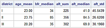
Apply different aggregation methods to columns defined by the GroupBy object.
gb = df.groupby(['District'])
gb.agg({'Age' : 'mean',
     'Before' : 'median',
      'After' : ['sum', 'median', 'std']
       })
           Age Before After
          mean median   sum median   std
District
I        23.00     34   225  41.00 45.54
II       23.75     85   356  84.50 26.62
III      20.20     35   302  69.00 30.20
In example above the agg function is applied to the gb GroupBy object with a dictionary identifying differing aggregation methods for the columns. Recall a dictionary is a data structure holding key/value pairs. To perform multiple statistics on a column, pass a list of methods as the values to the dictionary.
The SAS analog.
proc summary data=df nway;
   class district;
   output out=gb_sum (drop = _TYPE_ _FREQ_)
          mean(age)       = age_mean
          median(before)  = bfr_median
          sum(after)      = aft_sum
          median(after)   = aft_median
          std(after)      = aft_std;
run;

proc print data = gb_sum noobs;
run;
Filtering by Group
Filter data based on a group’s statistic. First, display the DataFrame.
print(df)
   District Sector      Name  Before  After  Age
0         I  North    Patton      17     27   22
1         I  South    Joyner      13     22   19
2         I   East  Williams     111    121   29
3         I   West     Jurat      51     55   22
4        II  North      Aden      71     70   17
5        II  South    Tanner     113    122   32
6        II   East   Jenkins      99     99   24
7        II   West    Milner      15     65   22
8       III  North     Chang      69    101   21
9       III  South     Gupta      11     22   21
10      III   East   Haskins      45     41   19
11      III   West     LeMay      35     69   20
12      III   West     LeMay      35     69   20
Next, define the std_1 function to slice the rows where the standard deviation for age is less than 5.
def std_1(x):
   return x['Age'].std() < 5
Then apply the filter to the df DataFrame grouped by District by chaining the .filter method with the std_1 function as an argument.
df.groupby(['District']).filter(std_1)
   District Sector      Name  Before  After  Age
0         I  North    Patton      17     27   22
1         I  South    Joyner      13     22   19
2         I   East  Williams     111    121   29
3         I   West     Jurat      51     55   22
8       III  North     Chang      69    101   21
9       III  South     Gupta      11     22   21
10      III   East   Haskins      45     41   19
11      III   West     LeMay      35     69   20
12      III   West     LeMay      35     69   20
GroupBy for Continuous Values
Group by the Age column which has continuous values. Use a dictionary to define the stats function for returning the statistics.
def stats(group):
    return {'count' : group.count(),
            'min'   : group.min(),
            'max'   : group.max(),
            'mean'  : group.mean()}
Define the bins object where the first group is 0 - 25, second is 26 - 50 and so on and define the corresponding gp_labels object.
bins = [0, 25, 50, 75, 200]
gp_labels = ['0 to 25', '26 to 50', '51 to 75', 'Over 75']
Assign ‘cut-points’ to the bins object as a list of values for the upper and lower bounds of the bins created with the cut method. Assign these results to the new Age_Fmt column in the df DataFrame.
df['Age_Fmt'] = pd.cut(df['Age'], bins, labels=gp_labels)
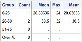
Use the apply method with the stats function to apply the statistics to column values for each group. The unstack method reshapes the returned object from a stacked form (in this case a Series to an unstacked form (a “wide” DataFrame).
df['Age'].groupby(df['Age_Fmt']).apply(stats).unstack()
          count   max  mean   min
Age_Fmt
0 to 25   11.00 24.00 20.64 17.00
26 to 50   2.00 32.00 30.50 29.00
51 to 75   0.00   nan   nan   nan
Over 75    0.00   nan   nan   nan
The SAS analog.
proc format cntlout = groups;
   value age_fmt
      0  - 25   = '0-25'
      26 - 50   = '26-50'
      51 - 75   = '51-75'
      76 - high = 'Over 75';

proc sql;
   select fmt.label label = 'Group'
        , count(dat.age) label = 'Count'
        , min(dat.age)   label = 'Min'
        , max(dat.age)   label = 'Max'
        , mean(dat.age)  label = 'Mean'
   from groups as fmt
      left join df as dat
         on fmt.label = put(dat.age, age_fmt.)
   group by fmt.label;
quit;
Transform Based on Group Statistic
Up to this point the GroupBy objects return DataFrames with fewer rows than the original. This is expected since GroupBy objects commonly perform aggregations. There are cases where one needs to apply a transformation based on group statistics and merge the transformed version with the original DataFrame.
Consider calculating a z-scores by creating a lambda expression as an anonymous function to compute values for rows within each group using the group’s computed mean and standard deviation.
z = df.groupby('District').transform(lambda x: (x - x.mean()) / x.std())
DataFrames allow the same name for multiple columns. So the rename attribute is applied to the z DataFrame passing a dictionary of key/value pairs where the key is the old column name and the value is the new column name.
Fetch the column names.
print(z.columns)
Index(['Before', 'After', 'Age'], dtype='object')
Rename the columns.
z = z.rename \
     (columns = {'Before' : 'Z_Bfr',
                 'After'  : 'Z_Aft',
                 'Age'    : 'Z_Age',
                })
Call the concat method to merge the df and z DataFrames. Additional concat examples are in the data managements section of this site.
df1 = pd.concat([df, z], axis=1)
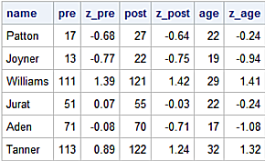
Output decimals two places and display the display the first six rows.
pd.options.display.float_format = '{:,.2f}'.format
print(df1[['Name', 'Before', 'Z_Bfr', 'After', 'Z_Aft', 'Age', 'Z_Age']].head(6))
       Name  Before  Z_Bfr  After  Z_Aft  Age  Z_Age
0    Patton      17  -0.68     27  -0.64   22  -0.24
1    Joyner      13  -0.77     22  -0.75   19  -0.94
2  Williams     111   1.39    121   1.42   29   1.41
3     Jurat      51   0.07     55  -0.03   22  -0.24
4      Aden      71  -0.08     70  -0.71   17  -1.08
5    Tanner     113   0.89    122   1.24   32   1.32
The program in a single go.
z = df.groupby('District').transform(lambda x: (x - x.mean()) / x.std())
print(z.columns)

z = z.rename \
     (columns = {'Before' : 'Z_Bfr',
                 'After'  : 'Z_Aft',
                 'Age'    : 'Z_Age',
                })
df1 = pd.concat([df, z], axis=1)
pd.options.display.float_format = '{:,.2f}'.format
print(df1[['Name', 'Before', 'Z_Bfr', 'After', 'Z_Aft', 'Age', 'Z_Age']].head(6))
Expressed as a SAS program.
proc summary nway data = df;
   class district;
   var pre
       post
       age;
   output out=z_out (drop = _TYPE_ _FREQ_)
          mean(age)  = age_mean
          mean(pre)  = pre_mean
          mean(post) = post_mean
          std(age)   = age_std
          std(pre)   = pre_std
          std(post)  = post_std;
run;

proc sort data = df presorted;
   by district;

run;

proc sort data = z_out presorted;
   by district;
run;

data z_df (drop = age_mean pre_mean post_mean
                  age_std  pre_std  post_std);
   merge df
         z_out;
   by district;

z_pre  = (pre - pre_mean)   / pre_std;
z_post = (post - post_mean) / post_std;
z_age  = (age - age_mean)   / age_std;
format z_pre z_post z_age 8.2;

run;

proc print data=z_df(obs=6) noobs;
   var name
       pre
       z_pre
       post
       z_post
       age
       z_age;
run;
Pivot
pandas provide the pivot_table function to create speadsheet-style pivot tables enabling aggregation of data across row and column dimensions.
Read the input data calling the read_csv method and call the info() function to view column metadata. Multiple examples of the the read_csv method are located in the pandas Readers & Writers section.
import pandas as pd
url = "https://raw.githubusercontent.com/RandyBetancourt/PythonForSASUsers/master/data/Sales_Detail.csv"
df2 = pd.read_csv(url, na_filter = False)
df2.info()
<class 'pandas.core.frame.DataFrame'>
RangeIndex: 2823 entries, 0 to 2822
Data columns (total 10 columns):
OrderNum       2823 non-null int64
Quantity       2823 non-null int64
Amount         2823 non-null float64
Status         2823 non-null object
ProductLine    2823 non-null object
Country        2823 non-null object
Territory      2823 non-null object
SalesAssoc     2823 non-null object
Manager        2823 non-null object
Year           2823 non-null int64
dtypes: float64(1), int64(3), object(6)
memory usage: 220.6+ KB
Call the pivot_table method for the df2 DataFrame, index the Year and ProductLine columns on the rows, index Territory on the columns and aggregate the Amount column.
df2.pivot_table(index   = ['Year', 'ProductLine'],
                columns = ['Territory'],
                values  = ['Amount'])
Territory             APAC     EMEA       NA
Year ProductLine
2016 Classic Cars 3,523.60 4,099.44 4,217.20
     Motorcycles  3,749.53 3,309.57 3,298.12
     Planes       3,067.60 3,214.70 3,018.64
     Ships             nan 3,189.14 2,827.89
     Trains       1,681.35 2,708.73 2,573.10
     Trucks       3,681.24 3,709.23 3,778.57
     Vintage Cars 2,915.15 2,927.97 3,020.52
2017 Classic Cars 3,649.29 4,062.57 3,996.12
     Motorcycles  2,675.38 3,736.90 3,649.07
     Planes       2,914.59 3,047.34 3,645.51
     Ships        2,079.88 3,030.86 3,067.40
     Trains            nan 3,344.41 2,924.96
     Trucks       3,695.36 4,344.76 3,326.99
     Vintage Cars 3,399.04 2,998.96 3,662.24
Notice row labels are formed using the Year column as the outer level and ProductLine as the inner level. Index arguments to the pivot_table function create either an index if one column is specified or a MultiIndex object if multiple columns are specified.
Replace the default aggregation with np.mean aggregation for columns by summing the Quantity column and averaging the Amount column. Call the fill_value argument to replace nan's with 0 (zero). Supply the margins=True argument to get row and column totals.
import numpy as np
pd.pivot_table(df2,values     = ['Amount', 'Quantity'],
                   columns    = 'Territory',
                   index      = ['Year', 'ProductLine'],
                   fill_value = 0,
                   aggfunc    = {'Amount'  : np.mean,
                                'Quantity' : np.sum},
                                 margins=True)
                        Amount                                        Quantity
Territory                 APAC         EMEA           NA          All     APAC   EMEA     NA    All
Year ProductLine
2016 Classic Cars  3523.597037  4099.436842  4217.195652  4106.951145      842   9152   5673  15667
     Motorcycles   3749.530000  3309.571562  3298.123385  3361.024797      683   2265   2105   5053
     Planes        3067.596923  3214.703898  3018.643913  3122.067034      419   2106   1582   4107
     Ships            0.000000  3189.140541  2827.892187  3080.084434        0   2664   1075   3739
     Trains        1681.350000  2708.729167  2573.102727  2638.749444       33    846    409   1288
     Trucks        3681.235714  3709.233171  3778.568113  3733.731549      252   2974   1901   5127
     Vintage Cars  2915.145625  2927.966544  3020.519333  2965.105660     1022   4523   4300   9845
2017 Classic Cars  3649.291463  4062.572241  3996.115055  4005.964600     1484  10433   6408  18325
     Motorcycles   2675.384286  3736.899011  3649.072588  3655.500929      193   3401   3016   6610
     Planes        2914.592500  3047.343675  3645.514237  3226.593936      394   4015   2211   6620
     Ships         2079.880000  3030.862432  3067.396154  3030.845156       56   2526   1806   4388
     Trains           0.000000  3344.409630  2924.959286  3201.182683        0    921    503   1424
     Trucks        3695.358077  4344.764828  3326.990533  3758.490314      926   2176   2548   5650
     Vintage Cars  3399.041176  2998.955663  3662.238403  3289.029498     1178   5631   4415  11224
All                3376.116878  3556.574365  3586.649339  3553.889072     7482  53633  37952  99067
For the rows examine Status within Year by Territory.
pd.pivot_table(df2,values     = ['Amount'],
                   columns    = ['Territory'],
                   index      = ['Year', 'Status'],
                   fill_value = 0,
                   aggfunc    = (np.sum))
                    Amount
Territory             APAC        EMEA          NA
Year Status
2016 Cancelled        0.00    48710.92        0.00
     Shipped     326991.61  2446585.86  1713727.25
2017 Cancelled        0.00   100418.90    45357.66
     In Process   43971.43    87329.98    13428.55
     On Hold          0.00    26260.21   152718.98
     Shipped     375158.79  2725139.76  1926828.95
SAS analog to produce the same report.
filename git_csv temp;
proc http
   url="https://raw.githubusercontent.com/RandyBetancourt/PythonForSASUsers/master/data/Sales_Detail.csv"
   method="GET"
   out=git_csv;

proc import datafile = git_csv
   dbms=csv
   out=sales_detail
   replace;
run;

proc sort data=sales_detail;
   by territory;
run;

proc summary data=sales_detail nway;
   by territory;
   class year
         status;
   var amount;
   output out=sales_sum (drop = _TYPE_ _FREQ_)
   sum(amount) = amount_sum;
run;

proc sort data = sales_sum;
   by year status;
run;

proc transpose data = sales_sum
                out = sales_trans(drop=_name_);
                id territory;
by year status;
run;

proc print data=sales_trans;
   var apac
       emea
       na;
id status
   year;
format apac
       emea
       na dollar13.2;
run;
