Introduction
In this section we cover common data management tasks like concatenation, updating, appending, sorting, finding duplicates, drawing samples, and transposing. Every analysis task requires data to be organized into a specific form before it renders meaningful results.
Update
SAS UPDATE operations are used in cases where a master table containing original data values are updated with smaller transaction datasets. Transaction datasets are typically shaped the same as the master containing new values for updating the master dataset. In the case of SAS, observations from the transaction dataset not corresponding to observations in the master dataset become new observations.
Create the SAS master and trans datasets.
data master;
   input ID
         salary;
list;
datalines;
023 45650
088 55350
099 55100
111 61625
;;;;
run;

data trans;
   infile datalines dlm=',';
   input ID
         salary
         bonus;
list;
datalines;
023, 45650, 2000
088, 61000,
099, 59100,
61625, 3000
121, 50000,
;;;;
run;
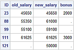
SAS UDAPTE operation creates the new_pay dataset applying transaction values from the transact dataset to the master dataset. Non-missing values for variables in the transact dataset replace corresponding values in the master dataset. A RENAME statement is used to rename the salary variable in order to display the effects of the UPDATE operation.
Updated master Dataset
The pandas update method modifies DataFrame values using non-NA values from another DataFrame. In contrast to SAS, the pandas update method performs an in-place update to the calling DataFrame, in this case the master DataFrame. The SAS UPDATE statement creates a new dataset and does not modify the master dataset.
Construct and print the master dataframe.
import pandas as pd
master = pd.DataFrame({'ID': ['023', '088', '099', '111'],
                   'Salary': [45650, 55350, 55100, 61625]})
print(master)
    ID  Salary
0  023   45650
1  088   55350
2  099   55100
3  111   61625
Contruct and print the trans dataframe.
import nump as np
trans = pd.DataFrame({'ID': ['023', '088', '099', '111', '121'],
           'Salary': [45650, 61000, 59100, 61625, 50000],
           'Bonus': [2000, np.NaN , np.NaN, 3000, np.NaN]})
print(trans)
    ID  Salary   Bonus
0  023   45650  2000.0
1  088   61000     NaN
2  099   59100     NaN
3  111   61625  3000.0
4  121   50000     NaN
Call the update method to update the master DataFrame values with those from the trans DataFrame and display the results.
master.update(trans)
print(master)
    ID  Salary
0  023   45650
1  088   61000
2  099   59100
3  111   61625
The default join operation for the update method is a left join explaining why row ID 121 is not in the updated master DataFrame. This row exists only in the trans DataFrame. This is also the explanation for why the Bonus column in the trans DataFrame is not updated for the master DataFrame.
Seems like we should be able to call the pandas update method with the join='outer' argument.
master.update(trans, join='outer')
NotImplementedError: Only left join is supported
The correct alternative is to call the merge method shown below.
df6 = pd.merge(master, trans,
               on='ID', how='outer',
               suffixes=('_Old','_Updated' ))
print(df6)
    ID  Salary_Old  Salary_Updated   Bonus
0  023     45650.0           45650  2000.0
1  088     55350.0           61000     NaN
2  099     55100.0           59100     NaN
3  111     61625.0           61625  3000.0
4  121         NaN           50000     NaN
The on='ID' argument uses the ID column common to the master and trans DataFrame as join keys. The how='outer' argument performs an outer join and suffixes=('_Old','_Updated' ) adds a suffix to liked-name columns in the DataFrames to disambiguate column contributions.
Conditional Update
There are cases when updates need to be applied conditionally. SAS users are accustomed to thinking in terms of IF/THEN/ELSE logic for conditional updates. To understand how the logic works with DataFrames we offer two examples.
The first example defines a Python function to calculate tax rates based on the Salary_Updated column in the df6 DataFrame. This example uses row iteration with Python if/else logic to calculate the new Taxes column.
Copy and the df6 DataFrame to df7, to be used in the second example and display the df6 DataFrame.
df7 = df6.copy()
print(df6)
    ID  Salary_Old  Salary_Updated   Bonus
0  023     45650.0           45650  2000.0
1  088     55350.0           61000     NaN
2  099     55100.0           59100     NaN
3  111     61625.0           61625  3000.0
4  121         NaN           50000     NaN
Define the calc_taxes function using if/else logic. To cascade a series of if statements use the elif statement following the first if statement.
def calc_taxes(row):
    if row['Salary_Updated'] <= 50000:
        val = row['Salary_Updated'] * .125
    else:
        val = row['Salary_Updated'] * .175
    return val
Call the apply method applying the calc_taxes function along the df6 columns using the the axis=1 argument.
df6['Taxes'] = df6.apply(calc_taxes, axis=1)
print(df6)
    ID  Salary_Old  Salary_Updated   Bonus      Taxes
0  023     45650.0           45650  2000.0   5706.250
1  088     55350.0           61000     NaN  10675.000
2  099     55100.0           59100     NaN  10342.500
3  111     61625.0           61625  3000.0  10784.375
4  121         NaN           50000     NaN   6250.000
The second approach is a better performing method using the loc indexer to apply calculated values to the DataFrame.
df7.loc[df7['Salary_Updated'] <= 50000, 'Taxes'] = df7.Salary_Updated * .125

df7.loc[df7['Salary_Updated'] >  50000, 'Taxes'] = df7.Salary_Updated * .175

print(df7)
    ID  Salary_Old  Salary_Updated   Bonus      Taxes
0  023     45650.0           45650  2000.0   5706.250
1  088     61000.0           61000     NaN  10675.000
2  099     59100.0           59100     NaN  10342.500
3  111     61625.0           61625  3000.0  10784.375
4  121         NaN           50000     NaN   6250.000
The two conditions are:
1. 12.5% tax rate on the Salary_Updated values less than or equal to 50,000 is:
df7.loc[df7['Salary_Updated'] <= 50000, 'Taxes'] = df7.Salary_Updated * .125
A way to read this statement is consider the syntax to the left of the comma (,) like a WHERE clause. The df7 DataFrame calls the loc indexer to slice rows where column df7['Salary_Updated'] values are less than or equal to 50,000.
To the right of the comma is the assignment when the condition is True; the values for the Taxes column (created on the DataFrame) are calculated at 12.5% of the value for the Salary_Updated column.
2. 17.5% tax rate on the Salary_Updated values greater than 50,000
df7.loc[df7['Salary_Updated'] > 50000, 'Taxes'] = df7.Salary_Updated * .175
works in a similar fashion.
The loc indexer creates a Boolean mask for the df7DataFrame and slices rows meeting the condition. For the condition, df7['Salary_Updated'] <= 50000, when the Boolean mask returns True values are multipled by .125. Likewise for the condition, df7['Salary_Updated'] > 50000 values are multiplied by 17.5.
Display the Boolean mask used to slice the df7 DataFrame conditionally.
nl = '\n'

print(nl,
      "Boolean Mask for 'Salary_Updated' <= 50000",
      nl,
      df7['Salary_Updated'] <= 50000,
      nl,
      "Boolean Mask for 'Salary_Updated' > 50000",
       nl,
      df7['Salary_Updated'] > 50000)
Boolean Mask for 'Salary_Updated' <= 50000
0    True
1    False
2    False
3    False
4    True
Name: Salary_Updated, dtype: bool
Boolean Mask for 'Salary_Updated' > 50000
0     False
1     True
2     True
3     True
4     False
Name: Salary_Updated, dtype: bool
SAS conditional update.
data calc_taxes;
   set new_pay;
if new_salary <= 50000 then
   taxes = new_salary * .125;

else taxes = new_salary * .175;
run;

proc print data=calc_taxes;
   id ID;
run;

Concatenation
The pandas library implements a concat method similar in behavior to the SAS SET statement. The concat method ‘glues’ DataFrames on row and column basis.
The concat method signature is:
pd.concat(objs, axis=0, join='outer', join_axes=None,
            ignore_index=False, keys=None, levels=None,
            names=None, verify_integrity=False,
            sort=None, copy=True)
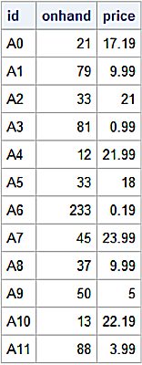
Construct loc1, loc2, and loc3 DataFrames. Call the concat method to concatenate them constructing the all DataFrame.
loc1 = pd.DataFrame({'Onhand': [21, 79, 33, 81],
                      'Price': [17.99, 9.99, 21.00, .99]},
                       index = ['A0', 'A1', 'A2', 'A3'])

loc2 = pd.DataFrame({'Onhand': [12, 33, 233, 45],
                      'Price': [21.99, 18.00, .19, 23.99]},
                       index = ['A4', 'A5', 'A6', 'A7'])

loc3 = pd.DataFrame({'Onhand': [37, 50, 13, 88],
                      'Price': [9.99, 5.00, 22.19, 3.99]},
                       index = ['A8', 'A9', 'A10', 'A11'])

frames = [loc1, loc2, loc3]
all = pd.concat(frames)

print(all)
     Onhand  Price
A0       21  17.99
A1       79   9.99
A2       33  21.00
A3       81   0.99
A4       12  21.99
A5       33  18.00
A6      233   0.19
A7       45  23.99
A8       37   9.99
A9       50   5.00
A10      13  22.19
A11      88   3.99
The analog SAS program.
data loc1;
   length id $ 3;
   input id $
         onhand
         price;
list;
datalines;
A0 21 17.19
A1 79 9.99
A2 33 21
A3 81 .99
;;;;
run;

data loc2;
   length id $ 3;
    input id $
          onhand
          price;
list;
datalines;
A4 12 21.99
A5 33 18
A6 233 .19
A7 45 23.99
;;;;
run;

data loc3;
   length id $ 3;
   input id $
          onhand
          price;
list;
datalines;
A8 37 9.99
A9 50 5
A10 13 22.19
A11 88 3.99
;;;;
run;

data all;

   set loc1
       loc2
       loc3;
run;
PROC SQL UNION ALL set operator as an alternative to the SET statement creating the all table.
proc sql;
   create table all as
   select * from loc1
      union all
   select * from loc2
      union all
   select * from loc3;

select * from all;
quit;
The concat method is able to construct a MultiIndex by providing the keys= argument to form the outermost level.
Construct the all DataFrame by concatenating loc1, loc2, and loc3 DataFrames. Construct the MultiIndex with the keys= argument.
all = pd.concat(frames, keys=['Loc1', 'Loc2', 'Loc3'])
print(all)
          Onhand  Price
Loc1 A0       21  17.99
     A1       79   9.99
     A2       33  21.00
     A3       81   0.99
Loc2 A4       12  21.99
     A5       33  18.00
     A6      233   0.19
     A7       45  23.99
Loc3 A8       37   9.99
     A9       50   5.00
     A10      13  22.19
     A11      88   3.99
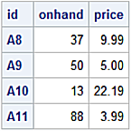
Call the loc indexer to slice rows where the outer-level index is 'Loc3'
all.loc['Loc3']
     Onhand  Price
A8       37   9.99
A9       50   5.00
A10      13  22.19
A11      88   3.99
An approximate SAS analog with the IN= dataset option.
data all;
length id $ 3;
   set loc1 (in=l1)
       loc2 (in=l2)
       loc3 (in=l3);
if l1 then location = 'Loc1';
if l2 then location = 'Loc2';
if l3 then location = 'Loc3';
run;

proc print data = all(where=(location='Loc3'));
   id id;
   var onhand
       price;
run;
Append
Similar to PROC APPEND the pandas library provisions an append method as a convenience to the concat method. The append method syntax is more natural for SAS users.
all_parts = loc1.append([loc2, loc3])
print(all_parts)
     Onhand  Price
A0       21  17.99
A1       79   9.99
A2       33  21.00
A3       81   0.99
A4       12  21.99
A5       33  18.00
A6      233   0.19
A7       45  23.99
A8       37   9.99
A9       50   5.00
A10      13  22.19
Call PROC APPEND to append observations from a dataset to a base dataset. In cases where more than one dataset is appended, multiple calls are needed. In some cases appending is a better performer over the SET statement when appending smaller datasets to a larger ones.
proc append base = loc1
            data = loc2;
run;

proc append base = loc1
            data = loc3;
run;

proc print data=loc1;
run;

Find Column Min and Max
pandas min and max methods return the minimum and maximum column values respectively.
all_parts['Price'].max()
23.99
all_parts['Price'].min()
0.19
Slice the row containing the highest price.
all_parts[all_parts['Price']==all_parts['Price'].max()]
    Onhand  Price
A7      45  23.99
PROC SQL returning column min and max.
proc sql;
   select min(price) as Price_min
        , max(price) as Price_max
from loc1;
quit;

Sort
pandas sort_values method and PROC SORT use ascending as their default sort order.
Construct the display the df DataFrame.
df = pd.DataFrame({'ID': ['A0', 'A1', 'A2', 'A3', 'A4', '5A', '5B'],
                  'Age': [21, 79, 33, 81, np.NaN, 33, 33],
                  'Rank': [1, 2, 3, 3, 4, 5, 6]})
print(df)
   ID   Age  Rank
0  A0  21.0     1
1  A1  79.0     2
2  A2  33.0     3
3  A3  81.0     3
4  A4   NaN     4
5  5A  33.0     5
6  5B  33.0     6
Call the pandas sort_values method and display results. Pass a list of column labels to the by= argument to request a multi-key sort.
df.sort_values(by=['Age', 'Rank'])
   ID   Age  Rank
0  A0  21.0     1
2  A2  33.0     3
5  5A  33.0     5
6  5B  33.0     6
1  A1  79.0     2
3  A3  81.0     3
4  A4   NaN     4
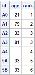
Construct the df dataset, request a multi-key sort with by age rank; and display the output.
data df;
   length id $ 2;
   input  id $
          age
          rank;
list;
datalines;
A0 21 1
A1 79 2
A2 33 3
A3 81 3
A4 .  4
5A 33 5
5B 33 6
;;;;

proc sort data = df;
   by age rank;
run;

proc print data = df;
   id id;
run;
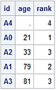
Dataset sorted by Age, Rank
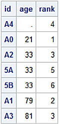
PROC SORT sorts missing values as the smallest numeric value. The default behavior for pandas sort_values method is to sort NaN’s as the largest numeric values. The sort_values method has the na_postion= argument with values 'first' or 'last' for placing NaN’s at the beginning or end of a DataFrame.
Sort NaN's to beginning of a DataFrame.
df.sort_values(by=['Age', 'Rank'], na_position='first')
   ID   Age  Rank
4  A4   NaN     4
0  A0  21.0     1
2  A2  33.0     3
5  5A  33.0     5
6  5B  33.0     6
1  A1  79.0     2
3  A3  81.0     3
For a multi-key sort using sort_values method, ascending or descending sort order is specified with the ascending= argument using True or False for the same number of values listed with the by= argument.
DataFrame multi-key sort ascending for the Age column and descending for the Rank column.
df.sort_values(by=['Age', 'Rank'], na_position='first', ascending = (True, False))
   ID   Age  Rank
4  A4   NaN     4
0  A0  21.0     1
6  5B  33.0     6
5  5A  33.0     5
2  A2  33.0     3
1  A1  79.0     2
3  A3  81.0     3
PROC SQL uses the DESCENDING keyword following a column name to indicate a descending sort order used with an ORDER BY clause.
proc sql;
   select * from df
   order by age
           ,rank descending;
quit;
Find Duplicates
In some cases data entry errors lead to duplicate data values or non-unique key values or duplicate rows. The duplicated method return Booleans indicating duplicate rows and, in this case, limited to duplicate values in the Age column. By default the duplicated method applies to all DataFrame columns.
print(df)
   ID   Age  Rank
0  A0  21.0     1
1  A1  79.0     2
2  A2  33.0     3
3  A3  81.0     3
4  A4   NaN     4
5  5A  33.0     5
6  5B  33.0     6
Create a Boolean mask to find all occurrences of duplicate values for Age excluding the first occurrence.
dup_mask = df.duplicated('Age', keep='first')
df_dups = df.loc[dup_mask]
print(df_dups)
   ID   Age  Rank
5  5A  33.0     5
6  5B  33.0     6
The statement:
dup_mask = df.duplicated('Age', keep='first')
defines a Boolean mask using the keep='first' argument for the duplicated attribute. The keep= argument can have three values:
- first: Mark duplicates as True except for the first occurrence
- last: Mark duplicates as False except of the last occurrence
- false: Mark all duplicates as True
Drop Duplicates
The drop_duplicates method returns a de-duplicated DataFrame based on argument values.
Display the df DataFrame.
print(df)
0  A0  21.0     1
1  A1  79.0     2
2  A2  33.0     3
3  A3  81.0     3
4  A4   NaN     4
5  5A  33.0     5
6  5B  33.0     6
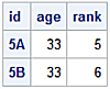
Call the drop_duplicates method and drop the rows where there are duplicate values for the Age column excluding the first occurence and display the new de_duped DataFrame.
df_deduped = df.drop_duplicates('Age', keep = 'first')
print(df_deduped)
   ID   Age  Rank
0  A0  21.0     1
1  A1  79.0     2
2  A2  33.0     3
3  A3  81.0     3
4  A4   NaN     4
The NODUPKEY and NODUPRECS options for PROC SORT detect and remove duplicate values. The NODUPKEY option removes observations with duplicate BY values. This is analogous to the pandas drop_duplicates method with a column argument.
The PROC SORT NODUPRECS is analogous to the drop_duplicates method with the keep=False argument. In each case, duplicate observations or rows, if found, are eliminated.
SAS Analog.
proc sort data = df nodupkey
   out = df_deduped
   dupout = df_dups;
   by age;

run;

proc print data = df;
   id id;
run;

proc print data = df_dups;
   id id;
run;

proc print data = df_deduped;
   id id;
run;
df Dataset
 df_dups Dataset
df_deduped Dataset
Draw Samples
Construct and display the df DataFrame using a seed value to make the results repeatable.
np.random.seed(987654)
df = pd.DataFrame({'value': np  .random.randn(360)},
     index=pd.date_range('1970-01-01', freq='M', periods=360))
print(df.head(5))
               value
1970-01-31 -0.280936
1970-02-28 -1.292098
1970-03-31 -0.881673
1970-04-30  0.518407
1970-05-31  1.829087
Create the samp1 DataFrame calling the sample method drawing a random sample of 100 rows from the df DataFrame without replacement.
samp1 = df.sample(n= 100, replace=False)
samp1.head(5)
               value
1993-10-31 -0.471982
1998-04-30 -0.906632
1980-09-30 -0.313441
1986-07-31 -0.872584
1975-01-31  0.237037
Return the number of rows and columns for the samp1 DataFrame.
print(samp1.shape)
(100, 1)
SAS Analog.
data df;
   do date = '01Jan1970'd to '31Dec2000'd by 31;
       value = rand('NORMAL');
       output;
   end;
format date yymmdd10.;
run;

data samp1 (drop = k n);
   retain k 100 n;
   if _n_ = 1 then n = total;
   set df nobs=total;

   if ranuni(654321) <= k/n then do;
      output;
      k = k -1;
   end;
n = n -1;

if k = 0 then stop;
run;
pandas sample method has the frac= argument to include a portion, for example, 30% of the rows to be included in the sample.
samp2 = df.sample(frac=.3, replace=True)
print(samp2.head(5))
               value
1971-05-31  0.639097
1997-10-31  1.779798
1971-07-31  1.578456
1981-12-31  2.114340
1980-11-30  0.293887
Convert Types
pandas provisions the astype method to convert column types. The DataFrame dtypes attribute returns the column’s type.
Construct the df8 DataFrame and return the column types.
df8 = pd.DataFrame({'String': ['2', '4', '6', '8'],
                    'Ints'  : [1, 3, 5, 7]})
df8.dtypes
String    object
Ints       int64
dtype: object
Convert the String column type from string to float and the Ints column type from integers to strings.
df8['String'] = df8['String'].astype(float)
df8['Ints']  = df8['Ints'].astype(object)
Get the altered column types for the df8 DataFrame.
df8.dtypes
String    float64
Ints       object
dtype: object
Rename Columns
Call the rename method to relabel columns using a dictionary with a key as the existing column label and the value as the new column label.
df8.rename(columns={"String": "String_to_Float",
                    "Ints": "Ints_to_Object"},
inplace=True)
print(df8)
String_to_Float Ints_to_Object
0              2.0              1
1              4.0              3
2              6.0              5
3              8.0              7
Map Values
Mapping column values is similar to the features provided by PROC FORMAT. Calling the map function allows translation of column values to corresponding values.
dow = pd.DataFrame({"Day_Num":[1,2,3,4,5,6,7]})
dow_map={1:'Sunday',
         2:'Monday',
         3:'Tuesday',
         4:'Wednesday',
         5:'Thursday',
         6:'Friday',
         7:'Saturday'
         }

dow["Day_Name"] = dow["Day_Num"].map(dow_map)
print(dow)
   Day_Num   Day_Name
0        1     Sunday
1        2     Monday
2        3    Tuesday
3        4  Wednesday
4        5   Thursday
5        6     Friday
6        7   Saturday
Transpose
Transposing creates a DataFrame by restructuring the values in a DataFrame transposing columns into row and rows into columns. Calling the T property is a convenience for the transpose method. Calling without arguments performs an in-place transpose.
uni = {'School'   :  ['NCSU',   'UNC',         'Duke'],
       'Mascot'   :  ['Wolf',   'Ram',         'Devil'],
       'Students' :  [22751,     31981,         19610],
       'City'     :  ['Raleigh', 'Chapel Hill', 'Durham']}
df_uni = pd.DataFrame(data=uni)
print (df_uni)
  School Mascot  Students         City
0   NCSU   Wolf     22751      Raleigh
1    UNC    Ram     31981  Chapel Hill
2   Duke   Devil    19610       Durham
Return the column types for the df_uni DataFrame.
df_uni.dtypes
School      object
Mascot      object
Students     int64
City        object
dtype: object
Create the new t_df_uni Dataframe by copying the transformed values.
t_df_uni = df_uni.T
print(t_df_uni)
                0            1       2
School       NCSU          UNC    Duke
Mascot       Wolf          Ram   Devil
Students    22751        31981   19610
City      Raleigh  Chapel Hill  Durham
Observe how all column types in the t_df_uni are returned as strings.
t_df_uni.dtypes
0    object
1    object
2    object
dtype: object
Slice column 0 (zero) with the [ ] operator.
t_df_uni[0]
School         NCSU
Mascot         Wolf
Students      22751
City        Raleigh
Name: 0, dtype: object
The SAS analog calling PROC TRANSPOSE.
data df_uni;
infile datalines dlm=',';
length school $ 4
mascot $ 5
city $ 11;
input school $
mascot $
students
city $;
list;
datalines;
NCSU, Wolf, 22751, Raleigh
UNC, Ram, 31981, Chapel Hill
Duke, Devil, 19610, Durham
;;;;
run;
proc print data = df_uni;
id school;
run;
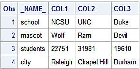
proc transpose data = df_uni
out = t_df_uni;
var school
mascot
students
city;
run;
proc print data = t_df_uni;
run;
Input Dataset

Transposed Dataset
Display the transposed dataset variable types fetching the result set from the SAS DICTIONARY.COLUMNS table.
proc sql;
   select name
        , type
   from dictionary.columns
where libname='WORK' and memname='T_DF_UNI';
quit;
Transposed Dataset column types
