DataFrame Index
SAS users tend to think of indexing SAS data sets to improve query performance or avoid dataset sorting. A SAS index stores values in ascending order for a specific variable or variables and manages information on how to locate a given observation(s) in the dataset.
pandas automatically creates an index structure at DataFrame creation time for both rows and columns. We ecountered the RangeIndex used as the default row index for DataFrame rows and columns. It is responsible for holding the axis labels and other metadata like integer-based location identifiers, axis names, etc.
Think of a DataFrame index as a means for labeling rows and columns. Recall that at DataFrame creation time, the RangeIndex object is created as the default index similar to the automatic _N_ variable SAS establishes at dataset creation time.
Just as you can return SAS dataset observations using the automatic variable _N_, a DataFrame's default RangeIndex return, or slice rows and columns using a zero-based offset.
Create Index
When a DataFrame is assigned an index, rows are accessible by supplying integer values from the RangeIndex as well the row or column label defined by an index.
Build and display the df Dataframe.
import pandas as pd
df = pd.DataFrame([['0071', 'Patton'  , 17,  27],
                   ['1001', 'Joyner'  , 13,  22],
                   ['0091', 'Williams', 111, 121],
                   ['0110', 'Jurat'   , 51,  55]],
         columns = ['ID',   'Name', 'Before', 'After'])
print(df)
         ID      Name  Before  After
    0  0071    Patton      17     27
    1  1001    Joyner      13     22
    2  0091  Williams     111    121
    3  0110     Jurat      51     55
Call the set_index method with the inplace=True argument and display the DataFrame with ID column as the index.
df.set_index('ID', inplace=True)
print(df)
          Name  Before  After
ID
0071    Patton      17     27
1001    Joyner      13     22
0091  Williams     111    121
0110     Jurat      51     55
Observe how the rows are now labeled with values from the ID column.
Indexers
Slice DataFrame rows or columns using three indexers.
1. [ ] operator enables selection by columns or by rows.
2. .loc indexer uses row and column labels for slicing. Column labels and row labels are assigned to an index, either with the index= parameter at DataFrame creation time or with the df.set_index method.
3. .iloc indexer uses integer positions (from 0 to length-1 of the axis) for sub-setting rows and columns provided by the default RangeIndex.
All indexers return a DataFrame.
Slice Columns by Position
Construct and print i DataFrame.
import pandas as pd
i = pd.DataFrame([['Patton'   , 17,  27],
                  ['Joyner'   , 13,  22],
                  ['Williams' , 111, 121],
                  ['Jurat'    , 51,  55],
                  ['Aden'     , 71,  70]])
print(i)
          0    1    2
0    Patton   17   27
1    Joyner   13   22
2  Williams  111  121
3     Jurat   51   55
4      Aden   71   70
Display the default RangeIndex for the rows and columns.
print(' Row Index: ', i.index, '\n', 'Column Index:', i.columns)
 Row Index:    RangeIndex(start=0, stop=5, step=1)
 Column Index: RangeIndex(start=0, stop=3, step=1)
Slice column 0 (zero).
i[0]
0      Patton
1      Joyner
2    Williams
3       Jurat
4        Aden
The [ ] operator accepts a Python list of columns, or rows to return. Recall a Python list is a mutable structure holding a collection of items. List literals are written within square brackets [ ] with commas (,) to indicate multiple list items.
Create the df DataFrame. Slice by placing the column labels Name and After in a list and display first 4 rows.
import pandas as pd
df = pd.DataFrame([['I','North', 'Patton', 17, 27],
                   ['I', 'South','Joyner', 13, 22],
                   ['I', 'East', 'Williams', 111, 121],
                   ['I', 'West', 'Jurat', 51, 55],
                   ['II','North', 'Aden', 71, 70],
                   ['II', 'South', 'Tanner', 113, 122],
                   ['II', 'East', 'Jenkins', 99, 99],
                   ['II', 'West', 'Milner', 15, 65],
                   ['III','North', 'Chang', 69, 101],
                   ['III', 'South','Gupta', 11, 22],
                   ['III', 'East', 'Haskins', 45, 41],
                   ['III', 'West', 'LeMay', 35, 69],
                   ['III', 'West', 'LeMay', 35, 69]],
                   columns=['District', 'Sector', 'Name', 'Before', 'After'])

df[['Name', 'After']].head(4)
       Name  After
0    Patton     27
1    Joyner     22
2  Williams    121
3     Jurat     55
The Python list with [' Name', 'After'] inside the DataFrame slice operator, [ ] results in two pair of brackets [ ]. The outer pair is the syntax for the DataFrame [ ] indexer while the inner pair hold the column names in a Python list.
SAS analog.
data df;
length sector $ 6
       name $ 8
       district $ 3;

infile cards dlm=',';
input district $
       sector $
       name $
       before
       after;
list;
datalines;
I,   North, Patton,   17,  27
I,   South, Joyner,   13,  22
I,   East,  Williams, 111, 121
I,   West,  Jurat,    51,  55
II,  North, Aden,     71,  70
II,  South, Tanner,   113, 122
II,  East,  Jenkins,  99,  99
II,  West,  Milner,   15,  65
III, North, Chang,    69,  101
III, South, Gupta,    11,  22
III, East,  Haskins,  45,  41
III, West,  LeMay,    35,  69
III, West,  LeMay,    35,  69
;;;;
run;

proc print data = df(obs=4);
   var name after;
run;
PROC PRINT output.

Slice Rows by Position
The syntax for the DataFrame [ ] indexer is:
df:[start : stop : step]
The start position is included in the output and the stop position is not. An empty start position implies 0 (zero).
df[:3]
District Sector      Name  Before  After
0        I  North    Patton      17     27
1        I  South    Joyner      13     22
2        I   East  Williams     111    121
Return every other row.
df[::2]
   District Sector      Name  Before  After
0         I  North    Patton      17     27
2         I   East  Williams     111    121
4        II  North      Aden      71     70
6        II   East   Jenkins      99     99
8       III  North     Chang      69    101
10      III   East   Haskins      45     41
12      III   West     LeMay      35     69
Return every other row with SAS.
data df1;
   set df;
if mod(_n_, 2) ^= 0 then output;
run;
NOTE: There were 13 observations read from the data set WORK.DF.
NOTE: The data set WORK.DF1 has 7 observations and 5 variables

Slice Rows and Columns by Position
The .iloc indexer uses integer positions (from 0 to length-1 of the axis) using the default RangeIndex to slice rows and columns. The syntax for the .iloc indexer is:
df.iloc[row selection, column selection]
Slice first and last row.
df.iloc[[0, -1]]
       District Sector    Name  Before  After
Name
Patton        I  North  Patton      17    100
LeMay       III   West   LeMay      35     69
SAS Analog.
data df1;
   set df end = last;

if name in ('Patton', 'Jurat', 'Gupta') then after = 100;
if _n_  = 1 then output;
if last = 1 then output;
run;

proc print data = df1 noobs;
run;
Slice Rows and Columns by Label
The .loc indexer is a method for returning rows and columns by labels.
To retrieve rows from the df DataFrame by label, set the Name column as the DataFrame index. This action assigns values from the Name column as labels for the rows.
Dislay the df DataFrame before index creation:
print(df)
   District Sector      Name  Before  After
0         I  North    Patton      17     27
1         I  South    Joyner      13     22
2         I   East  Williams     111    121
3         I   West     Jurat      51     55
4        II  North      Aden      71     70
5        II  South    Tanner     113    122
6        II   East   Jenkins      99     99
7        II   West    Milner      15     65
8       III  North     Chang      69    101
9       III  South     Gupta      11     22
10      III   East   Haskins      45     41
11      III   West     LeMay      35     69
12      III   West     LeMay      35     69
Call the .index attribute for DataFrame df.
print(df.index)
RangeIndex(start=0, stop=13, step=1)
Create the index in-place and display first 4 rows. drop=True drops the Name column from the DataFrame although it is still available to label rows.
df.set_index('Name', inplace = True, drop = True)
print(df.head(4))
         District Sector  Before  After
Name
Patton          I  North      17     27
Joyner          I  South      13     22
Williams        I   East     111    121
Jurat           I   West      51     55
Call the .index attribute to display the new index.
print(df.index)
Index(['Patton', 'Joyner', 'Williams', 'Jurat', 'Aden', 'Tanner', 'Jenkins','Milner', 'Chang', 'Gupta', 'Haskins', 'LeMay', 'LeMay'],
dtype='object', name='Name')
Using the index, slice the DataFrame. The syntax for the .loc indexer is:
df.loc[row selection, column selection]
Slice rows beginning with label Patton ending with label Aden inclusive. No value after the comma requests all columns.
df.loc['Patton': 'Aden', ]
         District Sector  Before  After
Name
Patton          I  North      17     27
Joyner          I  South      13     22
Williams        I   East     111    121
Jurat           I   West      51     55
Aden           II  North      71     70
Slice rows and columns. Column slice uses a list.
df.loc['LeMay', ['Before','After']]
       Before  After
Name
LeMay      35     69
LeMay      35     69
Conditional Slicing
Slice rows with Boolean operators where Sector equals West and Before greater than 20.
df.loc[(df['Sector'] == 'West') & (df['Before'] > 20)]
      District Sector  Before  After
Name
Jurat        I   West      51     55
LeMay      III   West      35     69
LeMay      III   West      35     69
Slice rows where values in the Name column ending in "r" by chaining the str.endswith method, keep columns District and Sector.
df.loc[df['Name'].str.endswith("r"), ['Name, District', 'Sector']]
KeyError: 'the label [Name] is not in the [index]'
This raises a KeyError since we dropped the Name column earlier. One remedy is reset the index, 'returning' Name as a column.
df.reset_index(inplace = True)
df.loc[df['Name'].str.endswith("r"), ['Name', 'District', 'Sector']]
     Name District Sector
1  Joyner        I  South
5  Tanner       II  South
7  Milner       II   West
A better approach: Keep the Name column as the index and chain the .str.endswith attribute to the .index attribute.
df.set_index('Name', inplace = True, drop = True)
df.loc[df.index.str.endswith('r'), ['District', 'Sector']]
       District Sector
Name
Joyner        I  South
Tanner       II  South
Milner       II   West
SAS analog.
proc sql;
   select name
         ,district
         ,sector
   from df
where substr(reverse(trim(name)),1,1) = 'r';
quit;

The <a href="https://pandas.pydata.org/pandas-docs/stable/reference/api/pandas.DataFrame.isin.html"isin attribute returns a Boolean indicating if a Python list of elements are values found in the target DataFrame column Sector.
df.loc[df['Sector'].isin(['North', 'South'])]
       District Sector  Before  After
Name
Patton        I  North      17     27
Joyner        I  South      13     22
Aden         II  North      71     70
Tanner       II  South     113    122
Chang       III  North      69    101
Gupta       III  South      11     22
SAS analog with the <a href="http://support.sas.com/documentation/cdl//en/sqlproc/69822/HTML/default/viewer.htm#n17vpypuojeg9zn1psc26z2ymju5.htm"IN condition.
proc sql;
   select *
   from df
where sector in ('North', 'South');
quit;

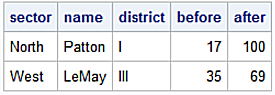
Updating with .loc Indexer
The .loc indexer can update values. Slice rows and columns before update.
df.loc[['Patton', 'Jurat', 'Gupta'], 'After']
Name
Patton    27
Jurat     55
Gupta     22
Name: After, dtype: int64
Update value for After column and display results.
df.loc[['Patton', 'Jurat', 'Gupta'], ['After']] = 100
df.loc[['Patton', 'Jurat', 'Gupta'], 'After']
Name
Patton    100
Jurat     100
Gupta     100
Name: After dtype: int64
SAS analog.
data df;
   set df;
   if _n_ = 1 then put
      'Name     After';

   if name in ('Patton', 'Jurat', 'Gupta') then do;
      after = 100;
      put @1 name @10 after;
   end;
run;
Name     After
Patton   100
Jurat    100
Gupta    100
MultiIndexing
This section introduces the DataFrame MultiIndex, also known as hierarchical indexing. Often the data for analysis is captured at the detail level. As part of performing an exploratory analysis, a MultiIndex DataFrame provides a multi-dimensional ‘view’ of data.
Call the DataFrame contructor method to create the tickets DataFrame. Set the idx row MultiIndex with Year as the outer-level and Month as the inner-level using the .from_product attribute. Set the columns MultiIndex with Area as the outer-level and When as the inner-level using the .from_product attribute.
import pandas as pd
import numpy as np
np.random.seed(654321)
idx = pd.MultiIndex.from_product([[2015, 2016, 2017, 2018],
                         [1, 2, 3]],
                 names = ['Year', 'Month'])
columns=pd.MultiIndex.from_product([['City' , 'Suburbs', 'Rural'],
                         ['Day' , 'Night']],
                 names = ['Area', 'When'])

data = np.round(np.random.randn(12, 6),2)
data = abs(np.floor_divide(data[:] * 100, 5))

tickets = pd.DataFrame(data, index=idx, columns = columns).sort_index().sort_index(axis=1)
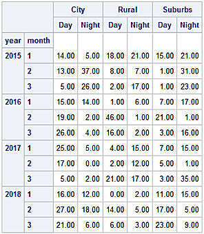
Display the tickets DataFrame.
print(tickets)
Area        City       Rural       Suburbs
When         Day Night   Day Night     Day Night
Year Month
2015 1      15.0  18.0   9.0   3.0     3.0   3.0
     2      11.0  18.0   3.0  30.0    42.0  15.0
     3       5.0  54.0   7.0   6.0    14.0  18.0
2016 1      11.0  17.0   1.0   0.0    11.0  26.0
     2       7.0  23.0   3.0   5.0    19.0   2.0
     3       9.0  17.0  31.0  48.0     2.0  17.0
2017 1      21.0   5.0  22.0  10.0    12.0   2.0
     2       5.0  33.0  19.0   2.0     7.0  10.0
     3      31.0  12.0  19.0  17.0    14.0   2.0
2018 1      25.0  10.0   8.0   4.0    20.0  15.0
     2      35.0  14.0   9.0  14.0    10.0   1.0
     3       3.0  32.0  33.0  21.0    24.0   6.0
Print the row Multi-index.
MultiIndex(levels=[[2015, 2016, 2017, 2018], [1, 2, 3]],
           codes=[[0, 0, 0, 1, 1, 1, 2, 2, 2, 3, 3, 3], [0, 1, 2, 0, 1, 2, 0, 1, 2, 0, 1, 2]],
           names=['Year', 'Month'])
To slice DataFrame rows refer to: [2015, 2016, 2017, 2018] as the outer level of the MultiIndex to indicate Year and: [1, 2, 3] as the inner level of the MultiIndex to indicate Month for row slicing.
To slice columns refer to: ['City', 'Rural', 'Suburbs'] as the outer levels of the of the MultiIndex to indicate Area and: ['Day', 'Night'] as the inner portion of the MultiIndex to indicate When for column slicing.
Create the analog ticketsdataset with PROC TABULATE to render data shaped like the tickets DataFrame. The Python and SAS code call different random number generators.
data tickets;
   length Area $ 7
          When $  9;
   call streaminit(123456);
   do year = 2015, 2016, 2017, 2018;
      do month = 1, 2, 3;
         do area = 'City', 'Rural', 'Suburbs';
            do when = 'Day', 'Night';
               tickets = abs(int((rand('Normal')*100)/5));
               output;
            end;
         end;
      end;
   end;
run;

proc tabulate;
   var tickets;;
   class area
         when
         year
         month;
   table year * month ,
         area=' ' * when=' ' * sum=' ' * tickets=' ';
run;
Slicing with MultiIndexes
A MultiIndex has the ability to slice by “partial” labels identifying data subgroups. Partial selection “drops” levels of the hierarchical index analogous to row and column slicing.
tickets['Rural']
When         Day  Night
Year Month
2015 1       9.0    3.0
     2       3.0   30.0
     3       7.0    6.0
2016 1       1.0    0.0
     2       3.0    5.0
     3      31.0   48.0
2017 1      22.0   10.0
     2      19.0    2.0
     3      19.0   17.0
2018 1       8.0    4.0
     2       9.0   14.0
     3      33.0   21.0
For each month how many tickets were issued in the city during night time?
tickets['City', 'Night']
Year  Month
2015  1        18.0
      2        18.0
      3        54.0
2016  1        17.0
      2        23.0
      3        17.0
2017  1         5.0
      2        33.0
      3        12.0
2018  1        10.0
      2        14.0
      3        32.0
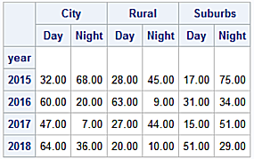
Create and print the sum_tickets DataFrame by applying the sum function to return the sum of all tickets by year.
sum_tickets = tickets.sum(level = 'Year')
print(sum_tickets)
Area   City        Rural      Suburbs
When   Day  Night  Day  Night Day  Night
Year
2015  31.0  90.0  19.0  39.0  59.0  36.0
2016  27.0  57.0  35.0  53.0  32.0  45.0
2017  57.0  50.0  60.0  29.0  33.0  14.0
2018  63.0  56.0  50.0  39.0  54.0  22.0
The SAS analog.
ods output
   table = sum_tickets (keep = area
                                when
                                year
                                tickets_sum);
proc tabulate data=tickets;
   var tickets;
   class area
         when
         year;
   table year,
         area=' ' * when=' ' * sum=' ' * tickets=' ';run;

ods output close;
proc print data = sum_tickets;
run;
Apply the sum function along a column.
sum_tickets2 = tickets.sum(level = 'Area', axis=1)
print(sum_tickets2)
Area        City  Rural  Suburbs
Year Month
2015 1      33.0   12.0      6.0
     2      29.0   33.0     57.0
     3      59.0   13.0     32.0
2016 1      28.0    1.0     37.0
     2      30.0    8.0     21.0
     3      26.0   79.0     19.0
2017 1      26.0   32.0     14.0
     2      38.0   21.0     17.0
     3      43.0   36.0     16.0
2018 1      35.0   12.0     35.0
     2      49.0   23.0     11.0
     3      35.0   54.0     30.0
Advanced Slicing with MultiIndexes
Slicing rows and columns with the .loc indexer can be used with a MultiIndexed DataFrame using similar syntax. It supports Boolean logic for filtering.
Slice rows for 2018 and return all columns.
tickets.loc[2018]
Area   City       Rural       Suburbs
When    Day Night   Day Night     Day Night
Month
1      25.0  10.0   8.0   4.0    20.0  15.0
2      35.0  14.0   9.0  14.0    10.0   1.0
3       3.0  32.0  33.0  21.0    24.0   6.0
Slice rows for month 3, year 2018 and all columns.
tickets.loc[2018, 3, :]
Area       City       Rural       Suburbs
When        Day Night   Day Night     Day Night
Year Month
2018 3      3.0  32.0  33.0  21.0    24.0   6.0
MultiIndex Slicing Rows and Columns
Slice the 3rd month for each year. Seems like the correct syntax.
tickets.loc[(:,3),:]
>>> tickets.loc[(:,3),:]
  File "<stdin>", line 1
    tickets.loc[(:,3),:]
                 ^
SyntaxError: invalid syntax
However, a : (colon) is illeage inside a tuple. As a convenience Python’s built-in slice(None) function selects all the content for a level. Let's try again.
tickets.loc[(slice(None), 3), :]
Area        City       Rural       Suburbs
When         Day Night   Day Night     Day Night
Year Month
2015 3       5.0  54.0   7.0   6.0    14.0  18.0
2016 3       9.0  17.0  31.0  48.0     2.0  17.0
2017 3      31.0  12.0  19.0  17.0    14.0   2.0
2018 3       3.0  32.0  33.0  21.0    24.0   6.0
The syntax slice(None) is the slicer for the Year column to include all values for a given level, in this case, 2015 to 2018 followed by 3 to designate the level for month. Empty values for the column selection using : (colon) returns all columns.
Slice months 2 and 3 for all years and no column slices.
tickets.loc[(slice(None), slice(2,3)), :]
 Area        City       Rural       Suburbs
When         Day Night   Day Night     Day Night
Year Month
2015 2      11.0  18.0   3.0  30.0    42.0  15.0
     3       5.0  54.0   7.0   6.0    14.0  18.0
2016 2       7.0  23.0   3.0   5.0    19.0   2.0
     3       9.0  17.0  31.0  48.0     2.0  17.0
2017 2       5.0  33.0  19.0   2.0     7.0  10.0
     3      31.0  12.0  19.0  17.0    14.0   2.0
2018 2      35.0  14.0   9.0  14.0    10.0   1.0
     3       3.0  32.0  33.0  21.0    24.0   6.0
Eventually we have difficulty supplying a collection of tuples for the slicers used by the .loc indexer. pandas provide the IndexSlice object to deal with this situation.
idx = pd.IndexSlice
tickets.loc[idx[2015:2018, 2:3], :]
Area        City       Rural       Suburbs
When         Day Night   Day Night     Day Night
Year Month
2015 2      11.0  18.0   3.0  30.0    42.0  15.0
     3       5.0  54.0   7.0   6.0    14.0  18.0
2016 2       7.0  23.0   3.0   5.0    19.0   2.0
     3       9.0  17.0  31.0  48.0     2.0  17.0
2017 2       5.0  33.0  19.0   2.0     7.0  10.0
     3      31.0  12.0  19.0  17.0    14.0   2.0
2018 2      35.0  14.0   9.0  14.0    10.0   1.0
     3       3.0  32.0  33.0  21.0    24.0   6.0
In the above example, tickets.loc[idx[2015:2018, 2:3], :] return years 2015:2018 inclusive on the outer level of the row MultiIndex and months 2 and 3 inclusive on the inner level. The : (colon) designates the start and stop positions for the row labels. Following the row slicer is a , (comma) designating the column slicer, in this case, all columns.
Request months 2 and 3 for year 2018 as the row slice with City and Rural from the Areaouter-level column slice.
idx = pd.IndexSlice
tickets.loc[idx[2018:, 2:3 ], idx['City', 'Day' : 'Night']]
Area        City
When         Day Night
Year Month
2018 2      35.0  14.0
     3       3.0  32.0
In the example above, the column slicer does not slice along the inner level of the MultiIndex for When.
MultiIndex Conditional Slicing
The .loc indexer can use a Boolean Mask for slicing based an criteria applied to values in the DataFrame.
Which months are the number of issued tickets in the city during day time exceeding 25? Create a Boolean mask representing a slicer and apply it to the tickets DataFrame.
mask = tickets[('City' ,'Day' )] > 25
tickets.loc[idx[mask], idx['City', 'Day']]
Year  Month
2017  3        31.0
2018  2        35.0
Name: (City, Day), dtype: float64
In the example above, rows are sliced conditionally by defined mask object. Columns are sliced using City from the outer-level Area and Day from the inner-level When.
The where attribute returns a DataFrame the same size as the original whose corresponding values are returned when the condition is True. When the condition is False, the default behavior is to return NaN's.
missing = "XXX"
tickets.where(tickets> 30, other = missing)
Area       City       Rural       Suburbs
When        Day Night   Day Night     Day Night
Year Month
2015 1      XXX   XXX   XXX   XXX     XXX   XXX
     2      XXX   XXX   XXX   XXX      42   XXX
     3      XXX    54   XXX   XXX     XXX   XXX
2016 1      XXX   XXX   XXX   XXX     XXX   XXX
     2      XXX   XXX   XXX   XXX     XXX   XXX
     3      XXX   XXX    31    48     XXX   XXX
2017 1      XXX   XXX   XXX   XXX     XXX   XXX
     2      XXX    33   XXX   XXX     XXX   XXX
     3       31   XXX   XXX   XXX     XXX   XXX
2018 1      XXX   XXX   XXX   XXX     XXX   XXX
     2       35   XXX   XXX   XXX     XXX   XXX
     3      XXX    32    33   XXX     XXX   XXX
Cross Section
DataFrames provision the xs cross section method to slice rows and columns from an indexed DataFrame or 'partial data' in the case of a MultiIndexed DataFrame.
tickets.xs((1), level='Month')
Area  City       Rural       Suburbs
When   Day Night   Day Night     Day Night
Year
2015  15.0  18.0   9.0   3.0     3.0   3.0
2016  11.0  17.0   1.0   0.0    11.0  26.0
2017  21.0   5.0  22.0  10.0    12.0   2.0
2018  25.0  10.0   8.0   4.0    20.0  15.0
The xs method works along a column axis.
tickets.xs(('City'), level='Area', axis = 1)
When         Day  Night
Year Month
2015 1      15.0   18.0
     2      11.0   18.0
     3       5.0   54.0
2016 1      11.0   17.0
     2       7.0   23.0
     3       9.0   17.0
2017 1      21.0    5.0
     2       5.0   33.0
     3      31.0   12.0
2018 1      25.0   10.0
     2      35.0   14.0
     3       3.0   32.0
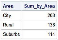
Sum of all issued tickets during daylight for each area.
tickets.xs(('Day'), level='When', axis = 1).sum()
Area
City       178.0
Rural      164.0
Suburbs    178.0
The SAS analog.
proc sql;
   select unique area
        , sum(tickets) as Sum_by_Area
   from tickets
       where when = 'Day'
   group by area;
quit;